Author: Y. Y.

  • How Much Are the World’s Oceans Really Warming? A New Method Finds a Large Gap With a Widely Used Climate Estimate — and Heat Moving Unevenly Between Ocean Basins

    How Much Are the World’s Oceans Really Warming? A New Method Finds a Large Gap With a Widely Used Climate Estimate — and Heat Moving Unevenly Between Ocean Basins

    • Almost all of the extra heat trapped by human-caused warming ends up in the ocean, so how well we can measure that heat shapes how much we can trust climate tracking and forecasts of rising seas.
    • German researchers built a new way to estimate that heat, combining data from floating ocean sensors and two kinds of satellites to recalibrate the computer reconstructions scientists normally rely on.
    • For part of the past two decades, one widely used reconstruction estimated far more ocean heat uptake than the new study did — in one stretch, nearly double.
    • The heat also hasn’t spread evenly: the Indian Ocean absorbed an outsized share between 2005 and 2015, a pattern that has since become more evenly spread across the Pacific, Indian, and Atlantic Oceans.

    Why the Ocean’s Heat Bill Matters

    Earth is currently taking in more heat from the sun than it radiates back out to space, mainly because greenhouse gases trap extra energy near the surface. Almost all of that surplus heat — roughly 90%, according to the new study — ends up in the ocean rather than in the air or on land. By absorbing so much of that excess energy, the ocean slows down how fast the atmosphere and land surface heat up, which is a large part of why it’s one of the most closely watched numbers in climate science.

    Scientists actually track two related but different numbers here: ocean heat content, meaning how much extra heat is already stored in the ocean, and ocean heat uptake, meaning how fast the ocean is gaining more of it, usually measured in watts per square meter of ocean surface. This story is mostly about the second number — the uptake rate, and how it differs from one ocean region to the next. As seawater heats up, it also expands slightly, a process called thermal expansion (think of a thermometer, where the liquid rises in the tube as it warms and takes up more space). That expansion drives a significant share of global sea-level rise.

    Getting a precise number for how fast the ocean is taking up heat, and where, turns out to be surprisingly hard. Researchers at the University of Bonn in Germany, in a study published in October 2026 in the journal Earth System Science Data, set out to make that accounting more reliable — and to see how it compares with the estimates climate scientists currently rely on.

    Three Data Sources, One Recalibrated Picture

    No one can scoop up the ocean and measure its heat directly. Scientists instead combine indirect clues, and each one has blind spots on its own. The Bonn team’s new approach, which they call GAAMR (Grace, Altimetry and Argo Mode Rescaling), draws on three streams of satellite and ocean data: two satellite-based measurements and one array of ocean-going floats.

    The first is a global fleet of thousands of drifting robotic sensors called Argo floats, which sink and rise through the upper two kilometers of the ocean roughly every ten days, recording temperature and salinity as they go; Argo samples the upper ocean far more densely than the deep ocean, so deeper water is handled differently, as explained below. The second is satellite radar altimetry, which tracks the height of the sea surface from orbit; averaged over time, it can measure global sea-level trends to within a couple of millimeters a year, and warmer water takes up more space, so part of that rise reflects ocean expansion. The third is data from GRACE, a pair of satellites that detect tiny shifts in Earth’s gravity field caused by moving mass on and near the surface, including ice sheets, glaciers, and water stored on land. That gravity data helps researchers separate the part of sea-level rise caused by this extra mass from the part caused by the ocean simply expanding as it warms.

    Importantly, the new method isn’t a model-free measurement. It still starts from an ocean model — the same ORAS5 reanalysis used for comparison below — to map out the likely regional patterns of warming. What’s different is that, rather than trusting those modeled patterns at face value or applying one global adjustment factor to the whole ocean, the researchers rescale the patterns region by region using the real satellite and float observations. That regional rescaling, instead of a single worldwide correction, is the method’s main innovation, and it produces monthly, region-by-region estimates of ocean heat uptake rather than one rough global figure.
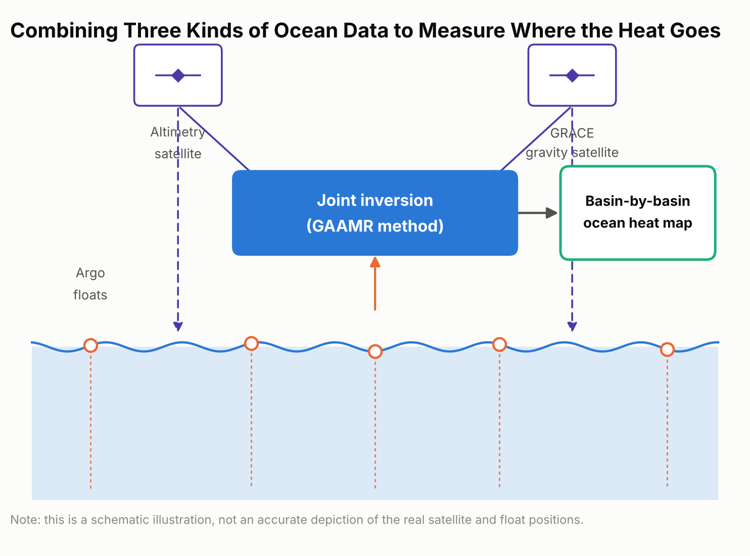
    Schematic diagram showing the three data sources combined in the GAAMR method: Argo floats, satellite altimetry, and GRACE gravity measurements
    The GAAMR method combines three data sources — Argo floats, satellite altimetry, and GRACE gravity data — to rescale ocean heat uptake estimates region by region.

    What the New Numbers Show

    Added up across the whole ocean, the new approach lines up reasonably well with several other independent estimates: it puts global ocean heat uptake from 2005 through 2024 at 0.62 watts per square meter, averaged over every patch of ocean surface on Earth. That figure is broadly consistent with estimates built from the Argo float network alone and with NASA’s CERES satellite measurements of Earth’s energy budget.

    Where the new estimate diverges is in comparison with ORAS5 specifically — a widely used “ocean reanalysis,” meaning a computer reconstruction that blends an ocean circulation model with whatever real-world observations are available, rather than a forward-looking climate projection. Over 2005–2024, ORAS5 put global ocean heat uptake at about 0.82 watts per square meter, roughly a third higher than the new study’s figure. The gap was much larger for the first half of that period.

    For 2005 to 2015, ORAS5 estimated ocean heat uptake at 1.09 watts per square meter, compared with 0.58 watts per square meter from the new GAAMR reconstruction — almost double.
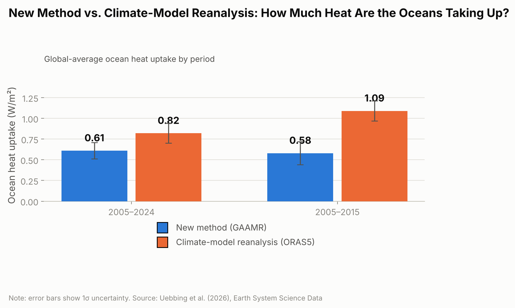
    Bar chart comparing ocean heat uptake in watts per square meter from ORAS5 and the new GAAMR method for 2005 to 2024 and 2005 to 2015
    For 2005 to 2015 alone, the gap between ORAS5 and the new GAAMR estimate is nearly twofold.

    The researchers are careful not to frame this as proof that climate models in general overstate ocean warming. Their own result broadly agrees with several independent observational estimates; the clearer gap is specifically with ORAS5, suggesting that particular reanalysis may be overstating how fast the ocean has taken up heat, especially during the 2005–2015 decade.

    Heat on the Move: Why Some Ocean Basins Differ

    The new regional estimates also reveal something a single global number can’t: heat hasn’t been spreading evenly across the world’s oceans. Over the full 2005–2024 period, the Pacific, Indian, and Atlantic Oceans together accounted for the large majority of the extra heat, with the Pacific absorbing the most, followed closely by the Indian Ocean and then the Atlantic. The Southern Ocean and Arctic Ocean, despite their size, contributed only a few percent combined.
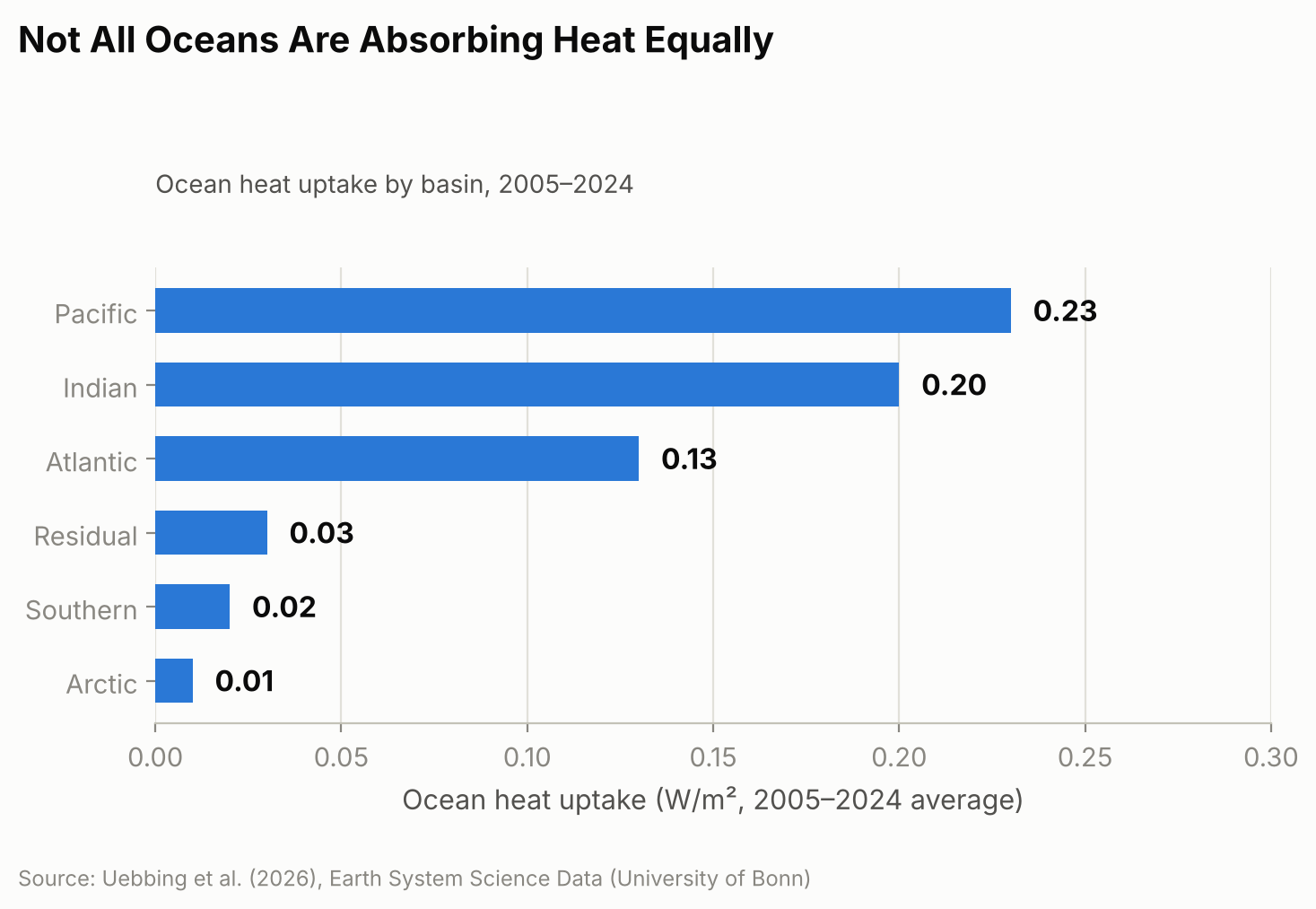
    Horizontal bar chart showing the regional breakdown of ocean heat uptake by basin for 2005 to 2024, covering the Pacific, Indian, Atlantic, Southern, and Arctic Oceans and a residual term
    The Pacific, Indian, and Atlantic Oceans together account for the large majority of the added heat.

    That balance, though, looks more even over 20 years than it did at the start. From 2005 to 2015, the Indian Ocean absorbed heat at a disproportionately high rate compared with its share of global ocean area. One contributor researchers point to is ocean circulation: heat transport patterns linked to the Indonesian Throughflow, a current system that channels warm Pacific water through the gaps between Indonesia’s islands into the Indian Ocean, appear to have shifted after around 2018, with larger outflows of heat carrying it away from the equatorial Indian Ocean. The study doesn’t pin down the mechanism conclusively, but that shift coincides with the broader move toward a more even split among basins that is clear in the full 20-year record. Other consequences of the same underlying warming are easier to see because they happen on land you can visit — this year’s near-record glacier melt across the Swiss Alps (the second-largest annual loss on record) is one example — even though the ocean, out of sight below the surface, is where almost all of the extra heat actually ends up.

    Why Getting This Number Right Matters

    Thermal expansion from ocean warming accounted for an estimated 42% of global sea-level rise between 1993 and 2015, according to the Intergovernmental Panel on Climate Change, and considerably more in some regions, so an inflated or understated ocean-heat figure can throw off coastal planning that depends on sea-level projections. The Bonn researchers also argue that ocean heat content is a steadier gauge of global warming than surface air temperature, which can swing sharply from a single hot or cool year in a way the ocean’s vast, slow-moving mass does not.

    The approach is not a forecasting tool — it’s a more careful reconstruction of what has already happened, built from twenty years of historical satellite and float records. The team says extending it further back in time is limited mainly by how sparse the satellite and ocean-observing records become before the early 1990s, and they plan to incorporate upcoming missions, including proposed successors to GRACE such as GRACE-C and NGGM, to keep the record going. They also call for sustained, internationally coordinated funding for the ocean- and gravity-monitoring satellites the method depends on, warning that gaps in that coverage would make it harder to catch the next shift in where the planet’s extra heat is headed.

    Sources: University of Bonn, “How Much Are the World’s Oceans Warming?”; Uebbing et al., “Improving global and regional ocean heat content by consistently combining GRACE gravity, satellite altimetry, and Argo profile observations in a joint inversion framework,” Earth System Science Data, 2026.
  • [Science] China’s Chang’e-6 Moon Samples Reveal a Rare Magnetic Mineral — A New Lead in the Mystery of the Moon’s Lost Protective Field

    [Science] China’s Chang’e-6 Moon Samples Reveal a Rare Magnetic Mineral — A New Lead in the Mystery of the Moon’s Lost Protective Field

    • Earth’s magnetic field acts like an invisible shield, deflecting much of the charged-particle wind that streams from the Sun — but the Moon and Mars both lost a global magnetic field like this billions of years ago, and scientists still do not fully agree on why.
    • Researchers studying soil that China’s Chang’e-6 mission brought back from the Moon’s far side found a rare, naturally magnetic form of iron that had never before been confirmed in real Moon rock.
    • Using a specialized microscope, they showed that this iron can hold a stable magnetic swirl pattern — the kind of structure that can, in principle, lock in a trace of the magnetic field present when it formed.
    • This is an early-stage finding: it does not by itself settle the long-running debate about the Moon’s lost magnetic field, but it gives scientists a new kind of physical evidence to test their ideas against.

    A missing magnetic shield, and a Moon that might hold a clue

    Right now, a layer of invisible magnetism generated deep inside Earth is quietly doing one of the most important jobs for life on this planet: deflecting much of the charged-particle wind that streams from the Sun, known as the solar wind, so it does not gradually strip away our atmosphere. Mars does not have this shield anymore. Neither does the Moon. Both are thought to have had one billions of years ago, generated by a “dynamo” — a churning flow of molten or partly molten metal inside the planet that behaves like a natural electric generator. Figuring out when and why each dynamo switched off is one of the open questions in planetary science, partly because it is also a preview of how a rocky world’s interior can change over very long timescales.

    The Moon is a convenient place to study this, because unlike Mars, it is close enough that spacecraft have brought real samples home. In 2024, China’s Chang’e-6 mission did something no previous mission had: it collected soil from the Moon’s far side, from the Apollo basin inside the giant South Pole–Aitken impact basin. A team at the Hefei Institutes of Physical Science (HFIPS), part of the Chinese Academy of Sciences, has now reported a new discovery hiding inside that soil, published online September 16, 2026, in the Proceedings of the National Academy of Sciences (PNAS).

    An iron that “shouldn’t” exist — until an asteroid hit made it

    The team, led by Prof. Haifeng Du, was looking at tiny beads of impact glass: droplets of rock that melted and then froze solid within moments after an asteroid or other object slammed into the Moon’s surface. Scattered through that glass, they found nanometer-scale particles — far smaller than a speck of dust, ranging from under 10 nanometers to about 140 nanometers across — made of a form of iron called gamma-iron, or γ-Fe for short.

    Gamma-iron is not exotic chemistry; it is simply metallic iron arranged in a different crystal structure than the form most people picture. At ordinary pressure, pure iron normally settles into a structure called alpha-iron as it cools, and that is the arrangement found in most familiar iron-rich rocks. Gamma-iron is normally only stable over a high-temperature range, roughly 912°C to 1,394°C, and should flip back into the ordinary form well before reaching room temperature. Finding it “frozen” in place at room temperature, inside real Moon soil, was unexpected. The researchers propose that the extremely rapid cooling that follows a high-speed impact — far faster than rock cools under ordinary conditions — combined with the small amount of trace elements in the particles, trapped the iron in this unusual structure before it had a chance to transform.

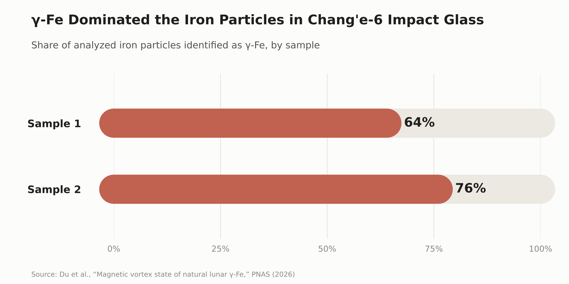
    Among 50 iron particles the team examined across two impact-glass samples, γ-Fe was the dominant crystal phase: it accounted for roughly 64% of the particles analyzed in one sample and 76% in the other. The particles also contained very little nickel, below 0.8% by weight, which helps distinguish them from the iron-nickel alloys already known from meteorites and other Moon rocks.

    Bar chart showing the share of analyzed iron particles identified as gamma-iron in two Chang’e-6 impact-glass samples: 64% and 76%.
    γ-Fe was the dominant iron phase in both impact-glass samples the team analyzed in detail.

    Reading a magnetic memory under the microscope

    Finding an unusual mineral is interesting on its own, but the more important part of the discovery is what the iron does magnetically. Using a specialized imaging technique called off-axis electron holography — a way of directly visualizing magnetic structure at a scale of billionths of a meter, inside an electron microscope — the team found that γ-Fe particles larger than about 100 nanometers settle into a stable “single-vortex” magnetic state: the magnetization inside the particle curls around in a stable loop, rather than pointing in one simple direction.

    That stability matters. A magnetic structure that holds its shape reliably, and responds in a predictable way to outside magnetic fields, is the kind of structure that can carry what scientists call remanent magnetization — a lasting trace of the magnetic field present when the material formed and cooled. In principle, that makes it somewhat like certain magnetic minerals in Earth’s own rocks, which preserve a record of our planet’s past magnetic field. Dr. Long Li, one of the researchers on the team, put it this way:

    “This tiny magnetic fossil may help us better understand the Moon’s ancient magnetic history.” — Dr. Long Li, Hefei Institutes of Physical Science

    It is worth being precise about what has, and has not, been shown so far. The team has demonstrated that γ-Fe exists in real lunar material, that it forms a stable magnetic vortex state, and that this state is capable of recording magnetization. What is not yet established is which magnetic field any particular particle actually recorded — the Moon’s ancient, planet-wide dynamo field, or a brief, local field generated by the heat and shock of the very impact that formed the glass bead around it. Telling those two signals apart is exactly the next step the researchers say this discovery opens up.

    A genuinely unsettled debate about the Moon’s lost magnetism

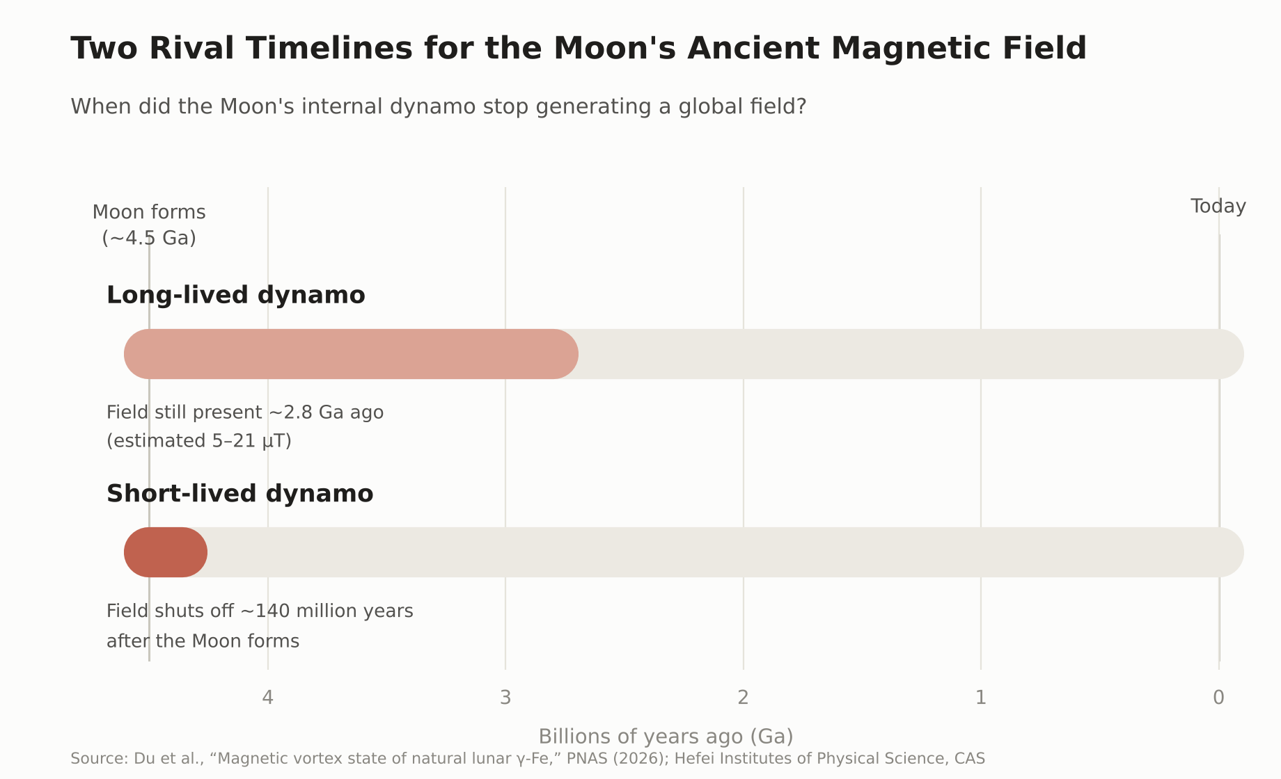
    Scientists already have evidence the Moon once had a working dynamo, because older Moon rocks brought back decades ago by the Apollo missions carry their own trace of ancient magnetism. Exactly how strong that field was, and especially how long it lasted, is still disputed — and this is a real, ongoing scientific disagreement rather than a settled fact with one outlier view. Paleomagnetic measurements of Chang’e-6 basalt reported a field of roughly 5 to 21 microtesla as recently as about 2.8 billion years ago, a result some researchers read as pointing toward a longer-lived dynamo. Other researchers, using different measurement methods on Apollo-era samples, have argued that the evidence for a long-lived global field is weaker than it first appeared, and that the core dynamo may have been largely confined to the Moon’s first 140 million years or so, with anything recorded afterward reflecting brief, impact-generated fields rather than a steady, planet-wide one.

    Timeline diagram comparing two rival hypotheses for when the Moon’s internal dynamo stopped generating a global magnetic field.
    Two competing timelines for when the Moon’s ancient dynamo shut off — a debate γ-Fe could eventually help settle.

    This is where γ-Fe could eventually contribute. Because it forms under different conditions than the more common alpha-iron, and appears specifically in impact-formed glass, comparing what it and other magnetic minerals “remember,” across many more samples, may eventually help researchers test whether a given signal reflects the Moon’s global dynamo, an impact-generated field, or some mixture of the two.

    Still early days: what comes next

    The team has not announced a new, confirmed timeline for when the Moon’s dynamo turned off, and γ-Fe on its own cannot provide a precise date for that event. What they have shown is that this magnetic mineral exists in real lunar material, that it can hold a stable magnetic state at the nanometer scale, and that it is a promising new tool for a field that has had to work with a frustratingly small and ambiguous set of physical clues. More broadly, understanding how a rocky world like the Moon or Mars generates, and eventually loses, its own internal magnetic field is part of a wider effort to understand what shapes a planet’s long-term climate and atmosphere — knowledge that also feeds into how scientists assess the conditions on rocky planets orbiting other stars. A small, newly identified mineral will not settle that larger question by itself, but it gives researchers one more concrete thread to pull on.

    Sources: Du, H. et al., “Magnetic vortex state of natural lunar γ-Fe,” PNAS (2026) · Hefei Institutes of Physical Science, CAS · ScienceDaily · The Brighter Side of News

  • [Science] Stimulating the Vagus Nerve After Practice Helps Mice Learn Better Days Later — Tohoku University Finds a Link to Rhythmic Changes in Brain Blood Volume

    [Science] Stimulating the Vagus Nerve After Practice Helps Mice Learn Better Days Later — Tohoku University Finds a Link to Rhythmic Changes in Brain Blood Volume

    • Applying electrical stimulation to the “vagus nerve” on the left side of the neck right after practicing something new may make mice better at it days later, a new study suggests.
    • If a similar effect holds in humans, it could eventually point toward new ways to support motor learning or rehabilitation.
    • Tohoku University researchers stimulated the vagus nerve while tracking local blood-volume changes in the brain, and found that repeated stimulation produced rhythmic fluctuations in local blood volume.
    • Mice with larger blood-volume oscillations after stimulation tended to score higher on a learning test five days later. This is a mouse study, though, and it’s not yet known whether the same effect would occur in humans.

    The Vagus Nerve — a Key Line Between Brain and Body

    The vagus nerve is a major nerve that runs from the brainstem through the neck, chest, and abdomen, carrying signals between the brain and organs such as the heart, lungs, and digestive tract. It’s one of the main nerves connecting the brain and internal organs in both directions: it carries signals about the body’s internal state — such as heart rate, breathing, and digestion — up to the brain, while also carrying signals from the brain back down to those organs.

    A treatment that stimulates this nerve from the outside with electrical pulses is called “vagus nerve stimulation,” or VNS. Using an implanted device, it’s an established therapy for epilepsy that doesn’t respond well enough to medication. In recent years, researchers have also been studying a non-invasive approach that stimulates part of the ear through the skin — though that’s a different method from the one used in this mouse study. Exactly what VNS changes inside the brain has remained unclear.

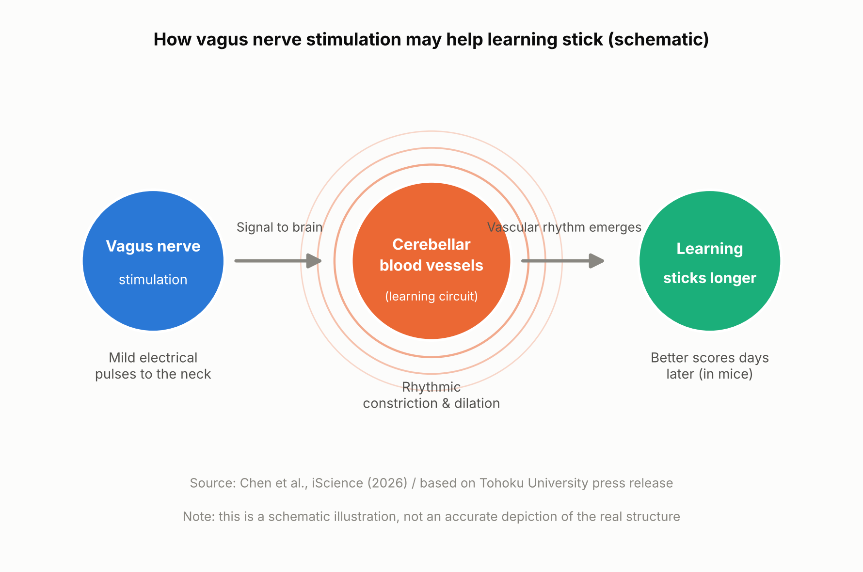
    Schematic showing how vagus nerve stimulation and a brain blood-volume rhythm relate to long-term learning
    How vagus nerve stimulation and a brain blood-volume rhythm relate to long-term learning (schematic illustration, not an accurate depiction of the real structure).

    The Mouse Experiment: Stimulation Came After Practice

    A team at Tohoku University’s Graduate School of Life Sciences — Junyu U. Chen, Assistant Professor Yoko Ikoma, and Professor Ko Matsui — fitted a small cuff electrode around the left cervical vagus nerve in mice and delivered electrical stimulation. The mice practiced a task called the horizontal optokinetic response (HOKR): tracking a vertical striped pattern that moved back and forth in front of them with their eyes. This kind of task is known to depend heavily on the cerebellum, a brain region central to motor learning.

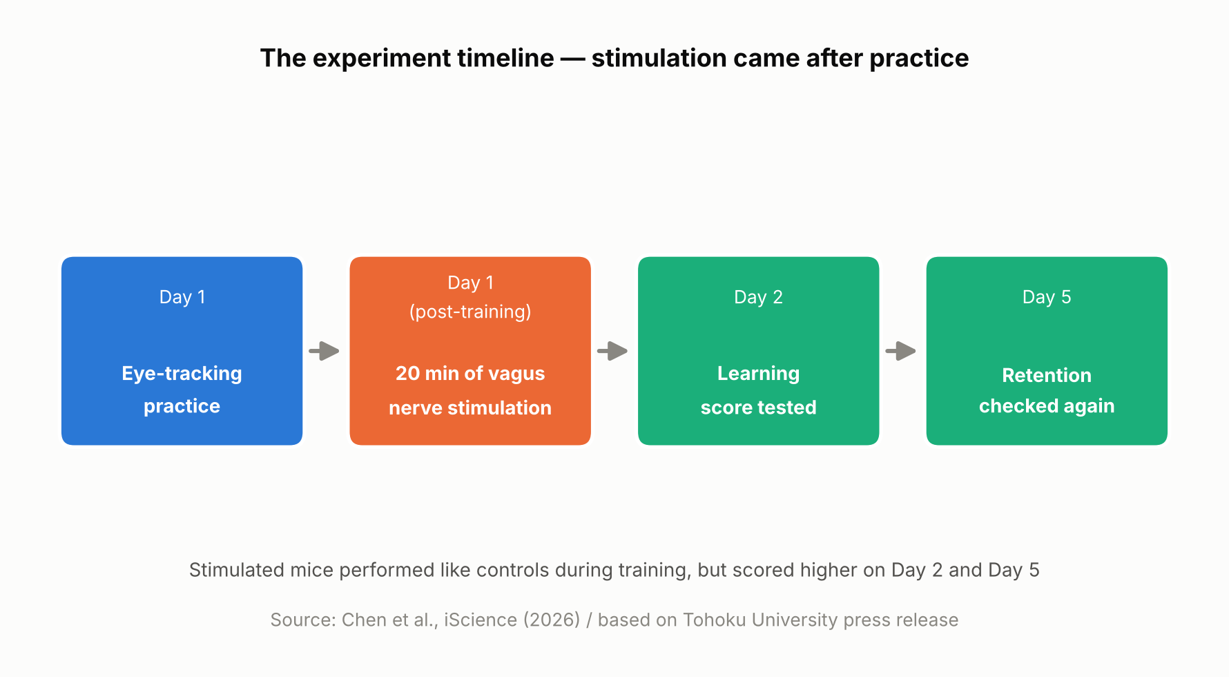
    On day one, the mice practiced for 15 minutes, four times, spaced an hour apart. Right after each day-one training session, mice in the stimulated group received 20 minutes of vagus nerve stimulation at one of two intensities, while control mice received none. Performance was then measured again on day two and day five.

    On day one itself, there was no difference between the stimulated and unstimulated mice. But by day two and especially day five, the stimulated mice showed higher scores, with the higher-intensity stimulation producing a visible benefit as early as day two and both intensities showing an advantage by day five. In other words, VNS didn’t directly boost performance during training — it appears to have improved later-day learning through some process that unfolded after training ended.

    Timeline of the mouse experiment, showing stimulation delivered after practice
    The experiment timeline. Based on Chen et al., iScience (2026) and the Tohoku University press release.

    Blood Volume Around the Cerebellum Fell Into Rhythm After Stimulation

    Using a light-based technique called fiber photometry, the researchers measured local blood-volume changes in tissue around the cerebellar flocculus. Each train of vagus nerve stimulation produced a two-step change: local blood volume briefly dipped, then — after a short delay — rose. This pattern is consistent with alternating contraction and dilation of blood vessels in that area.

    With repeated stimulation, this rise-and-fall pattern settled into a steady rhythm. The researchers think this rhythmic change in blood volume may be related to how the brain regulates local blood flow and its metabolic environment — but the study did not directly measure oxygen, ATP, or other metabolic markers, so exactly how the blood-volume rhythm might support learning is still unclear.

    Long-term learning is thought to involve various changes in the brain, including “synaptic plasticity” — changes in the connections and activity between neurons — which requires energy. The research team’s idea is that if the blood-volume rhythm is tied to how well-nourished brain tissue is, it could be helping support those changes, though this remains a hypothesis rather than something the study directly confirmed.

    Mice with larger blood-volume oscillations after stimulation tended to score higher on the learning test five days later

    A Bigger Rhythm, Better Long-Term Learning — but Only a Correlation So Far

    The most notable finding was a relationship between the magnitude of the blood-volume oscillations in the 20 minutes right after stimulation and performance five days later: mice with larger oscillations tended to score higher on day five. It’s worth being clear that this is a correlation, not proof that the blood-volume change caused the better learning.

    “The key point is that VNS was delivered only after training,” said Professor Matsui. “Our findings suggest that VNS may open a hidden window of opportunity for enhanced learning by making the brain environment more receptive to long-lasting change.” Lead author Junyu Chen added, “Our brains may be more strongly influenced by the body than we imagine. By tuning the brain’s metabolic environment, including rhythmic vascular movements, we may eventually unlock capacities that would otherwise remain latent.”

    What’s Still Unknown — and What Comes Next

    Based on this study alone, it’s not possible to say whether the blood-volume rhythm actually causes the learning improvement. Confirming that would require future experiments that directly manipulate blood-vessel or blood-volume activity and track the effect on learning. The researchers also did not directly measure metabolic molecules such as ATP, so the proposed mechanism remains a hypothesis.

    It’s also worth remembering that this was a mouse study using an invasive cuff electrode surgically placed around the cervical vagus nerve, delivering stimulation directly to the nerve rather than through the skin. Less invasive, ear-based stimulation methods are already being studied in humans for other purposes, but whether this mouse study’s results would carry over to humans — or to those non-invasive methods — can’t be determined from this result alone. The research team suggests that fine-tuning the timing and intensity of stimulation could eventually help support learning and rehabilitation, though that application remains a research goal rather than something available today.

    Sources: Tohoku University Graduate School of Life Sciences press release (August 26, 2026), Chen et al., iScience (published online August 25, 2026)

  • [Science] Scientists Build a Billion-Dalton Molecular Thread Longer Than a Cell — It Quadrupled Nerve-Cell Activity in the Lab

    [Science] Scientists Build a Billion-Dalton Molecular Thread Longer Than a Cell — It Quadrupled Nerve-Cell Activity in the Lab

    • A newly built, self-assembling material made nerve cells growing in a lab dish roughly four times more biologically active than usual, hinting that materials like it could one day help repair damaged nerves.
    • Chemists at Northwestern University found a new way to precisely control how long a certain kind of molecular thread grows, and how its positively and negatively charged segments are arranged along the way.
    • By molecular standards the resulting threads are enormous — roughly 100 times heavier than typical plastic-like polymers and bigger than even the largest proteins found in nature — even though they are built from many smaller molecules that click together on their own, rather than one molecule held together by ordinary chemical bonds.
    • So far the effect has only been shown in cells grown in a lab dish, not in animals or people, so any real treatment is still a long way off.

    Billion-Dalton Supramolecular Polymers: A Structure Big Enough to Rival a Cell

    A team led by the chemist Samuel I. Stupp at Northwestern University has built a new kind of giant structure, described in the journal Science on October 1, 2026. It belongs to a class of materials called supramolecular polymers. Rather than being a single molecule held together by strong chemical bonds the way an ordinary plastic is, it is made of many smaller molecules that click onto one another and hold themselves together more loosely, the way a line of magnets snaps together end to end. That looseness usually makes supramolecular polymers easy to assemble but hard to control, since there has been no reliable way to stop them from growing at a chosen point.

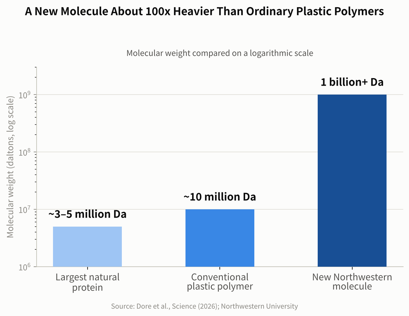
    Scientists weigh molecules in daltons, a unit named after the 19th-century chemist John Dalton, where one dalton is roughly the mass of a single hydrogen atom. Northwestern researchers point to common high-mass synthetic polymers used in materials science, which weigh around 10 million daltons, for comparison. Some of the largest proteins found in nature — the kind that give muscle tissue its structure — are in the roughly 3 to 5 million-dalton range. The new Northwestern assembly reaches a combined mass in the billions of daltons, around 100 times heavier than those conventional polymers, and its longest threads stretch farther than the width of a single living cell.

    Bar chart comparing molecular weight of a natural protein, a conventional polymer, and the new Northwestern assembly on a log scale
    Figure 1. Molecular weight on a log scale: a natural protein, a conventional polymer and the new billion-dalton supramolecular polymer. Source: data from Dore et al., Science (2026); Northwestern University

    Why Controlling the Length Was So Hard

    Because supramolecular polymers assemble themselves from many separate molecules rather than being built link by link under a chemist’s control, they have historically kept growing in a somewhat unpredictable way. That made it hard to control how long any given thread would grow, or where along its length particular features would end up. The Northwestern team solved this with a technique they call self-capping supramolecular polymerization: as the supply of available building-block molecules runs low, flexible regions at each end of the growing thread fold over on themselves, effectively capping the ends and stopping further growth.

    That trick let the researchers control two things at once: the overall length of each thread, and how positively and negatively charged segments are arranged along it. In a statement describing the work, Stupp called the result a breakthrough in materials design.

    “We discovered something we had never seen before in chemistry or in biology.”

    Precise Length and Charge Segmentation: The Charge Pattern Made the Difference

    Before arriving at their final design, the researchers tried several simpler charge patterns on neurons growing in a lab dish. Threads carrying only positive charge essentially killed the neurons; threads carrying only negative charge did almost nothing; and threads with positive and negative charge mixed randomly along their length produced no notable response either. Only one design worked well: a short positively charged segment flanked by longer negatively charged segments, arranged with precision rather than left to chance.

    To see how this winning design affected living neurons in culture, the researchers added it to cells growing in a lab dish and tracked them over 7 and 14 days. They used a technique called calcium imaging, which tracks what is known as calcium activity — a widely used indicator of how active a nerve cell is, since neurons briefly let calcium ions flow across their outer membrane as part of firing a signal. It is a standard, well-established way for researchers to gauge neural activity, though it is an indirect measure rather than a literal count of signals fired.

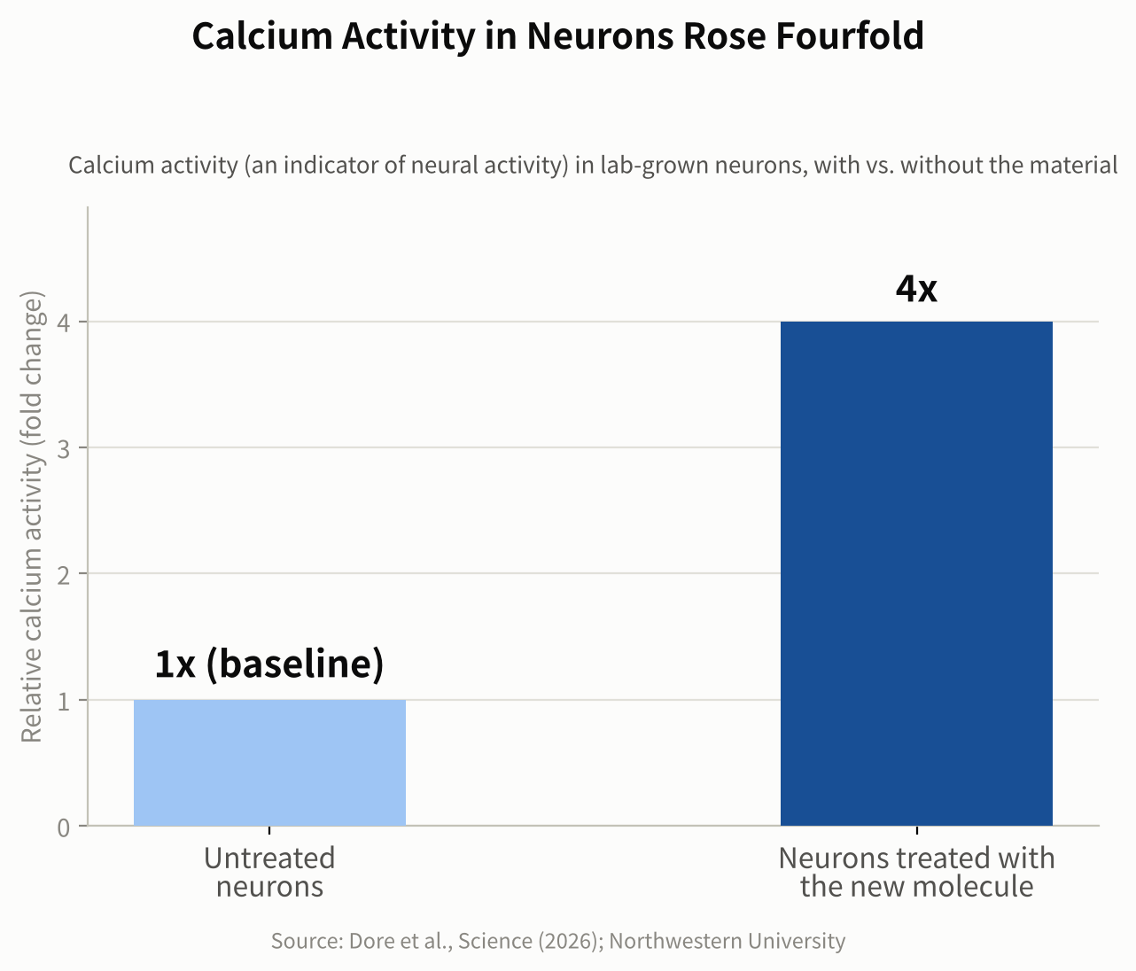
    Neurons treated with the winning design showed overall calcium activity roughly four times greater than untreated neurons after seven days, and had formed more synapses by 14 days. The researchers propose that the precise charge pattern works by shaping how the material interacts with the neurons’ outer membrane and with proteins around it, though they describe this as a proposed mechanism rather than a fully confirmed one. Notably, the effect appeared without adding any separate drug, growth factor, or other biological signaling molecule — the geometry of the charge pattern alone was enough to measurably change how the cells behaved.

    That matters because nerve cells are known to rely on their electrical activity, along with other cues, to grow new branches and form synapses, the junctions where one neuron passes a signal to the next. Materials associated with more active, better-connected neurons are therefore of particular interest for regenerative medicine, the branch of science focused on helping the body rebuild tissue it has lost or damaged, including nerve tissue after an injury. The researchers describe the link between an entirely synthetic, self-assembling material and this kind of change in living cells as the most surprising part of the result.

    Bar chart showing neurons treated with the new material had four times the calcium activity of untreated neurons
    Figure 2. Neurons treated with the new material showed about four times the calcium activity of untreated neurons. Source: data from Dore et al., Science (2026); Northwestern University

    From a Lab Dish to a Possible Therapy

    So far this particular design has only been tested on neurons growing in a dish, not in animals or people, so any medical use is still likely years away. Lab-dish results are a long way from a treatment: cells in a dish do not have to survive inside a living body, fight off an immune response, or integrate with surrounding tissue the way they would after an actual injury. The Stupp lab has, however, spent years designing self-assembling materials aimed at nerve repair and tissue regeneration, and the researchers see this new level of precision as a step toward building more reliable, tunable materials for that purpose. A logical next stage would be testing whether the material remains safe and effective in animal models of nerve damage, before any human study could even be considered.

    The achievement also matters well beyond medicine. Being able to build a giant synthetic structure with a chosen length and a precisely controlled charge pattern opens the door to new materials with tunable mechanical or electrical behavior, useful in fields far from biology too. More broadly, it shows how self-assembly can be used to control a material’s properties over distances far larger than a single molecule — a step toward manufacturing matter with a level of precision that has mostly been limited, until now, to much smaller scales.

    Sources: Northwestern Now, EurekAlert!

    Paper: Dore, M. et al., “Precise length and charge segmentation of billion-dalton supramolecular polymers”, Science (2026).

    Related: new to the topic? Start with What Is a Supramolecular Polymer? A Simple Guide to How It Works.

  • [Science] A Pufferfish’s Umami Sensor Is Broader Than Ours — What Its Structure Reveals About Why Animals Taste the World Differently

    [Science] A Pufferfish’s Umami Sensor Is Broader Than Ours — What Its Structure Reveals About Why Animals Taste the World Differently

    • Different animals can end up finding very different things “delicious” — and new research shows part of the reason comes down to the exact molecular shape of their taste sensors.
    • A Japanese research team used the SPring-8 synchrotron facility to determine the structure of the ligand-binding region of an umami receptor from pufferfish — the part that recognizes taste molecules.
    • The human umami receptor is highly selective: it responds strongly to only one mirror-image form of its target amino acid, and barely at all to the other. The pufferfish receptor, the team found, responds to both.
    • This is so far a test-tube finding about how the receptor binds molecules, not direct proof of what a pufferfish actually tastes. The difference may be related to the pufferfish’s diet, and the discovery could eventually help with new seasonings or aquaculture feed.

    Why the Same Food Doesn’t Taste the Same to Every Animal

    Umami — alongside sweet, sour, salty, and bitter — is one of the five basic tastes. It’s the savory taste produced when a receptor on the tongue detects certain amino acids, most notably glutamate, the compound behind the savory taste of kombu seaweed and dried bonito flakes. A receptor is a protein that changes shape when a specific molecule binds to it, and that shape change is what sends a signal into the cell. Scientists have long pictured this as a “lock and key”: a molecule has to be the right shape to fit and trigger a response.

    It has been difficult to determine exactly why umami receptors differ between species, partly because their three-dimensional structures are technically difficult to solve. Until now, structures of these receptors had been determined for only a small number of species, leaving the molecular basis of these differences unclear — even though different animals clearly do not all find the same molecules appetizing.

    Capturing the Pufferfish Receptor’s Shape at SPring-8

    A research team led by Professor Atsuko Yamashita at the Institute for Protein Research, Osaka University, working with Meiji University, Okayama University, Science Tokyo, and RIKEN, used X-ray crystallography to determine the crystal structure of the ligand-binding domain of the Tas1r1/Tas1r3 receptor complex — the extracellular region where taste molecules bind — in the tiger pufferfish (Takifugu rubripes, known in Japan as torafugu).

    The work was carried out at SPring-8, a large synchrotron radiation facility in Hyogo Prefecture, Japan. By aiming X-rays at extremely small protein crystals and analyzing the resulting diffraction pattern, the team worked out the three-dimensional structure of the pufferfish receptor’s taste-binding region for the first time.

    A Receptor That Also Responds to the “Mirror Image”

    Amino acids found in nature can exist in two mirror-image forms, often described loosely as “left-handed” and “right-handed” — what chemists call L- and D-amino acids. The human umami receptor strongly recognizes only the left-handed form — the same form as L-glutamate, the umami compound in kombu — and responds only weakly, if at all, to the right-handed form. To humans, that right-handed form often tastes sweet rather than savory.

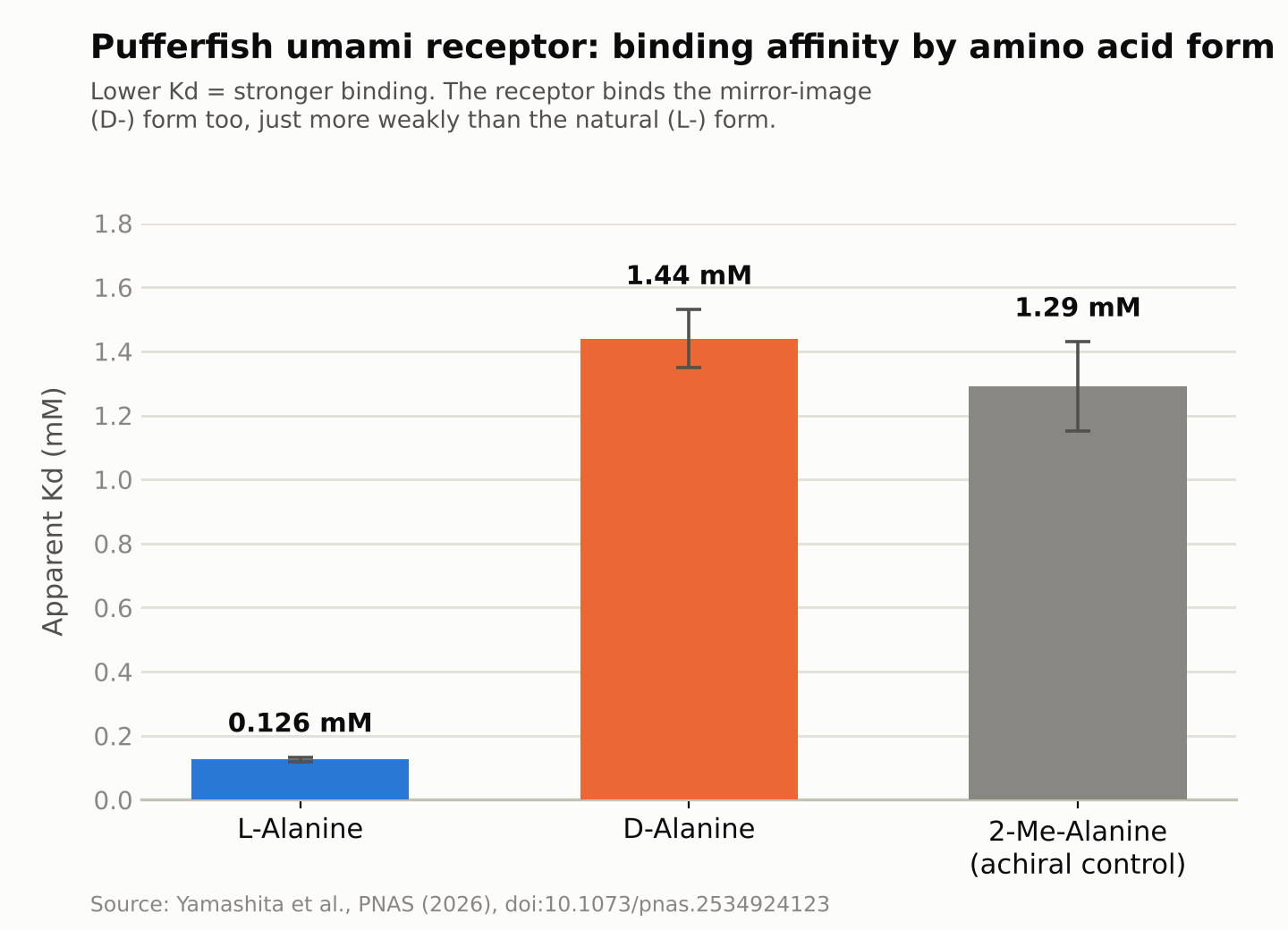
    The new study found that the pufferfish receptor binds, and sends a signal in response to, both forms. Measuring binding strength directly, the team found the receptor bound the left-handed form of the amino acid alanine strongly, at a concentration of about 0.126 millimolar, while it bound the right-handed form more weakly, at about 1.44 millimolar — roughly a tenfold difference. Weaker binding still triggered the receptor, though. It’s worth being precise about what this does and doesn’t show: the result demonstrates that the isolated receptor binds and signals in response to the right-handed molecule in a test tube. It does not, on its own, prove that a live pufferfish actually perceives that molecule as delicious.

    Bar chart comparing how strongly the pufferfish umami receptor binds left-handed versus right-handed amino acids
    Source: created from data in Yamashita et al., PNAS (2026). A lower value means stronger binding.

    A Molecular “Latch” That Holds the Receptor Shut

    The receptor resembles a two-lobed clamshell that closes around a bound molecule of the right shape, and that closing motion is what sends the taste signal. The right-handed amino acid doesn’t fit neatly into the human version of this receptor. When the team examined the pufferfish receptor’s structure closely, they found an additional set of interactions between the two lobes — acting like a molecular latch — that helps keep the binding cleft closed even when the bound molecule’s chirality doesn’t match the usual, better-fitting form. That latch appears to let the receptor keep signaling even while holding a right-handed amino acid that would otherwise bind too loosely to trigger a response.

    The researchers suggest that this broader receptor specificity may be related to the pufferfish’s diet: mollusks and crustaceans, which make up much of what it eats, contain relatively high amounts of right-handed (D-) amino acids. Whether pufferfish actually perceive these molecules as tasty in the way we understand taste is a separate question the receptor data alone cannot answer — but the researchers note it as a plausible evolutionary explanation for why the receptor tolerates both forms.

    Toward New Seasonings and Aquaculture Feed

    What the study shows is limited to the structure and binding behavior of an isolated receptor studied in the lab; it doesn’t directly confirm how a living pufferfish experiences taste. Still, the research institutions involved say the structural information could eventually be useful for designing new umami compounds suited to the human palate, or for developing feed that farmed fish and livestock find more palatable — a question worth attention in aquaculture, where improving feed acceptance can matter for production efficiency and cost. The team also says it hopes to compare receptor shapes across more species going forward, providing structural information that could eventually help develop AI models for predicting how taste receptors recognize different molecules.

    Sources: Meiji University press release, RIKEN press release, Mizoguchi, Toda, et al., PNAS (2026)

  • [Economy] Low Fertility Shows No Clear “Floor,” New Research Finds — What That Could Mean for Japan’s Shrinking Workforce

    [Economy] Low Fertility Shows No Clear “Floor,” New Research Finds — What That Could Mean for Japan’s Shrinking Workforce

    • If low fertility stays lower than some population projections assume, estimates of future workers, taxpayers, and pension contributors may need to be revised — a question that matters for anyone planning decades ahead.
    • Economists analyzed more than 70 years of global fertility data, plus detailed regional records from Japan, the United States, and India.
    • Across every dataset they checked — including all 47 of Japan’s prefectures — the researchers found no clear evidence of a stable, low fertility level at which decline reliably stopped.
    • This is a historical statistical pattern, not a guaranteed future: fertility could still stabilize in particular places, and the researchers themselves stress that this is about the evidence so far, not a prediction.

    A Question Buried Inside Every Population Forecast

    Long-range population projections produced by international organizations and government agencies sometimes build in a particular assumption: in countries where fertility has fallen very low, it will eventually stop declining and roughly stabilize — often somewhere near the “replacement” level, around 2.1 children per woman in a population with today’s typical mortality rates, the rough rate needed to keep a population steady over the long run without migration. Pension systems and long-term corporate planning often lean on projections like these, which is part of why the assumptions behind them matter.

    A new study tests that assumption against the historical record. In a National Bureau of Economic Research (NBER) working paper titled “Does Fertility Stabilize At Low Levels? Evidence from Period, Cohort, and Subnational Data,” economists Diane Coffey, Michael Geruso, Dean Spears, and Sangita Vyas ask a direct question: once fertility drops low, does it actually stop falling anywhere, or does it keep drifting down? Geruso and Spears also present a related analysis in a separate peer-reviewed article in the Journal of Economic Perspectives — a different paper, by two of the four authors, under a different title, rather than a peer-reviewed version of the same NBER study.

    Their conclusion: across the historical data, they found no robust evidence of a fertility level at which decline reliably stops or reverses. That holds globally, and it holds in the three countries — Japan, the United States, and India — where they examined the data region by region.

    Three Countries, One Shared Pattern

    The researchers combined three different kinds of evidence to examine the same question.

    First, they used “period” total fertility rate (TFR) data — a snapshot measure based on the fertility rates observed among women of different ages in a given year — for nearly every country in the world from 1950 to 2023, drawing on United Nations figures. Second, they looked at completed “cohort” fertility — the actual average number of children women in a given birth cohort had over their entire reproductive lives — using records for 31 countries, covering women born between 1935 and 1975. Third, they zoomed into regions within three countries: Japan’s 47 prefectures, individual U.S. states, and 351 districts in India.

    The same pattern showed up at every level. Worldwide, fertility fell from about five children per woman in 1950 to a little above two by 2023, and roughly two-thirds of the world’s population now lives in a country below the replacement level. Across the range of relatively low starting fertility levels in the data — from about 2.3 down to about 1.3 children per woman — the researchers found no point where fertility reliably flattened out afterward.

    In Japan, the median of the 47 prefectures’ fertility rates was 1.53 children per woman in 2015. From that starting point, fertility fell further over the next five years in each of Japan’s 47 prefectures, with no exceptions — not in prefectures that still had comparatively higher rates, and not in the ones that already had Japan’s lowest fertility.

    In U.S. states, the researchers found that, looking at data since 2010, fertility declined on average across every starting fertility level they examined. In India, where fertility is generally higher than in Japan or the U.S., the relationship between a district’s starting fertility and its subsequent change was negative across the entire range of 351 districts studied.

    A Counterintuitive Pattern: Declines Weren’t Slower Near Replacement

    One result stood out. If fertility really did settle near a natural equilibrium close to the replacement level, you might expect fertility sitting right around that level to decline more gently than fertility already well below it — the closer to a “floor,” the gentler the slope should be.

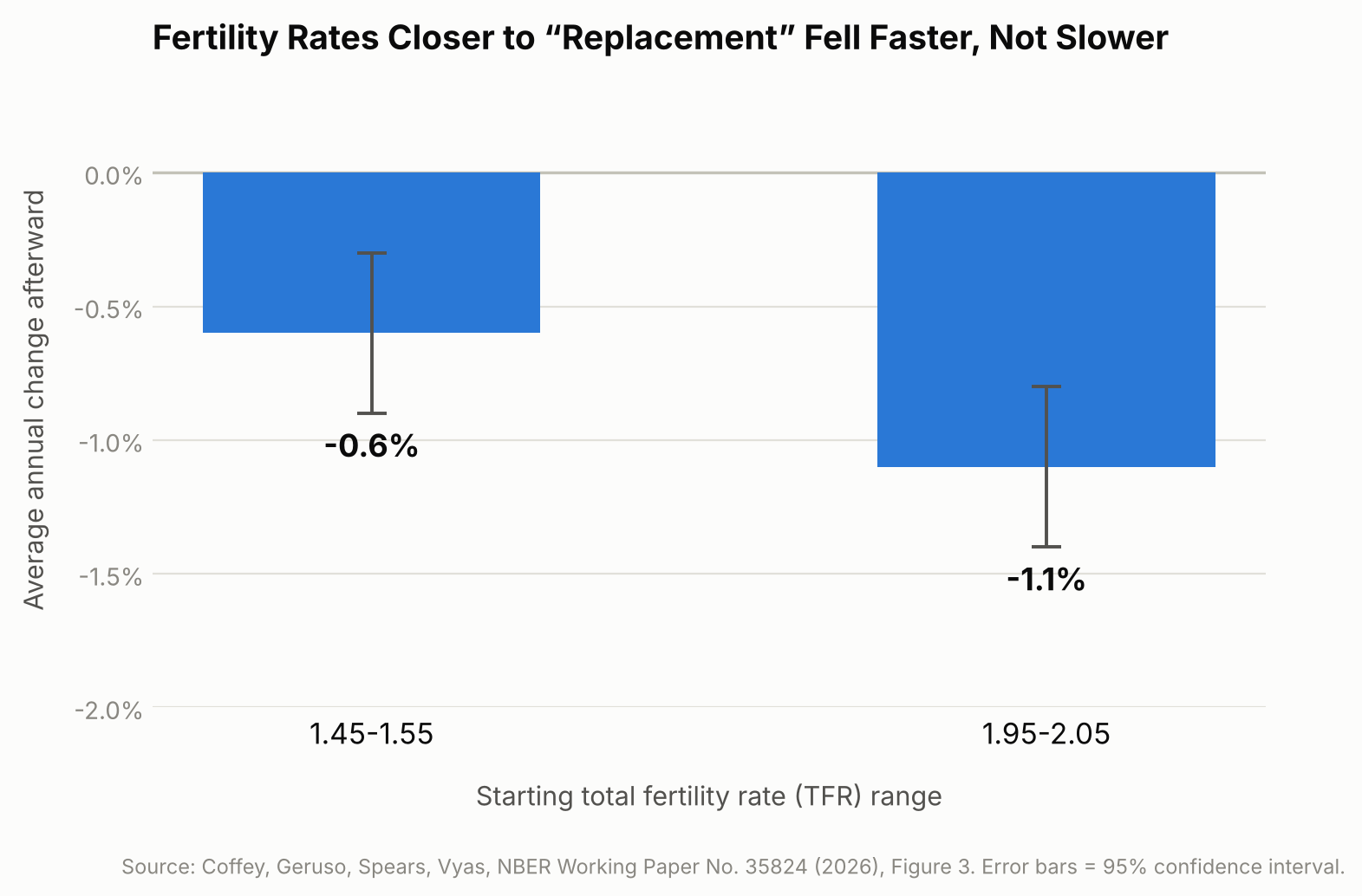
    A pattern where declines slow down as fertility approaches a “floor” did not show up. If anything, the opposite did. Looking at all the country-year observations worldwide from 1950 to 2023, the researchers calculated that fertility rates starting between 1.95 and 2.05 — almost exactly the replacement level — fell by an average of 1.1% per year afterward (a percentage change relative to the starting rate, not a drop of 1.1 children). Rates already lower, between 1.45 and 1.55, fell more slowly, by about 0.6% per year. This is a descriptive pattern in the historical data, not evidence that sitting near replacement fertility itself causes a faster decline; mainly, it argues against replacement level acting as a natural resting point for fertility.

    Bar chart showing fertility rates near replacement level fell faster than lower fertility rates
    Source: Coffey, Geruso, Spears, Vyas, NBER Working Paper No. 35824 (2026), Figure 3.

    Why This Matters Beyond Academic Debate

    This isn’t just an academic curiosity — it bears on economic planning. Pension systems, healthcare budgets, housing demand, and labor-force projections all rest on assumptions about how many future workers and taxpayers a country will have, and some population projections used by international and government agencies build in an assumption that fertility eventually stops falling.

    The study itself doesn’t forecast Japan’s future workforce, pension finances, or infrastructure needs — those depend on many other factors too, including life expectancy, retirement ages, labor-force participation, and migration. But if the historical pattern the researchers identify continues, projections that assume fertility will automatically stabilize may be worth re-examining in light of that pattern, which is relevant anywhere — Japan included — that is already planning for an aging, shrinking working-age population. The authors suggest that standard population projections are best read as conditional scenarios built on chosen assumptions, not as confident predictions of what will actually happen.

    The researchers write: “There is no robust evidence for a systematic fertility rebound, or for a stable equilibrium point at any fertility level conventionally assumed.”

    What This Research Doesn’t Tell Us

    A few limits matter here. First, this is a study of statistical patterns across the past, not a law of nature — it describes what has generally happened, not what must happen everywhere going forward; fertility could still stabilize or even rise in particular places. Second, the authors note that government programs designed to encourage childbirth can shift short-term “period” fertility statistics without necessarily changing how many children women ultimately have over their lifetimes — so a policy might appear to be working in a given year’s data without reversing the longer-run trend. Third, fertility decline and population decline are not the same thing: because of factors like population age structure and migration, a country’s workforce and total population can keep growing for years even after fertility drops below replacement, so the effects described here play out over decades, not immediately.

    Sources: NBER Working Paper No. 35824 (Coffey, Geruso, Spears, Vyas, 2026), Journal of Economic Perspectives, Vol. 40, No. 1 (Geruso & Spears, 2026)

  • [Science] APOE4 May Drive Scarring of Brain Blood Vessels — and a Human Brain-Tissue Model Showed the Process Can Be Reversed

    [Science] APOE4 May Drive Scarring of Brain Blood Vessels — and a Human Brain-Tissue Model Showed the Process Can Be Reversed

    • About one in four people carry a common gene variant that raises their odds of developing Alzheimer’s disease later in life — and scientists have now pinpointed, for the first time, exactly what that variant does to blood vessels in the brain.
    • The variant, called APOE4, is something people are simply born with; it isn’t caused by diet, exercise, or lifestyle.
    • Researchers found that APOE4 causes the cells that protect brain blood vessels to turn into “scar-forming” cells, making those vessels stiffer and more likely to clog.
    • The same team then found a way to brake that process in lab experiments, and even partly undo it.
    • The work is still limited to lab-grown tissue and animal models, but it points to a future where carrying this gene variant may not simply be something people have to live with — a treatment that slows or blocks the damage could eventually become possible.

    A Gene Long Blamed, Now Tied to a Specific Mechanism

    Scientists have linked APOE4 to Alzheimer’s since landmark studies in 1993, and subsequent research has implicated it in several disease-related processes, including amyloid-β metabolism and clearance, lipid handling, and inflammation. What has stayed less clear is exactly how APOE4 damages brain blood vessels, an abnormality long observed in carriers alongside the disease’s hallmark protein buildup. In a paper published in the journal Cell on September 24, 2026, a team led by Dr. Joel W. Blanchard at Mount Sinai pinned the vascular damage to a specific cell-identity switch, using evidence from human brain tissue, lab-grown human brain models, and mice.

    How a Support Cell Turns Into Scar Tissue

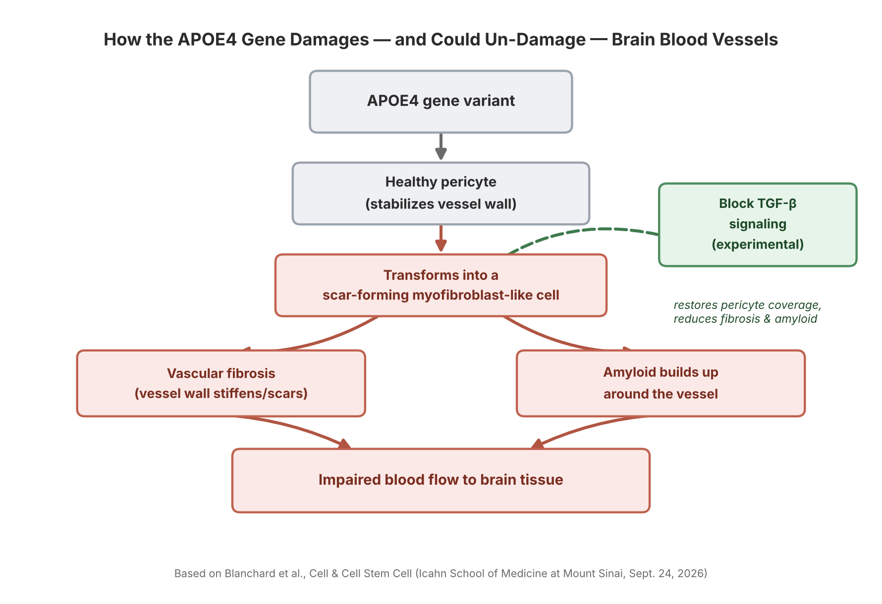
    Tiny blood vessels in the brain are wrapped in pericytes, cells that help stabilize the vessel wall and maintain the blood-brain barrier. The Mount Sinai team found that APOE4 pushes a portion of these pericytes into a myofibroblast-like state — a cell identity similar to the scar-forming cells involved in fibrosis in organs such as the liver and lungs. As more pericytes shift into this state, they produce a dense, fibronectin-rich extracellular matrix that accumulates in the vessel wall (a process called vascular fibrosis) and promotes the buildup of amyloid protein around the vessel. Mount Sinai’s own description of the work says these changes “may compromise blood flow” and contribute to neurodegeneration — a more cautious framing than saying blood flow is cut off outright, since that specific chain of cause and effect in people has not been directly demonstrated.

    Diagram: how APOE4 damages and could un-damage brain blood vessels
    Source: based on Blanchard et al., Cell & Cell Stem Cell (Icahn School of Medicine at Mount Sinai, Sept. 24, 2026)

    Built From Human Brain Tissue, Not Just Mice

    A notable part of this work is how closely it was tied to human biology. The researchers assembled a single-cell transcriptomic atlas of the human brain’s blood vessels, then examined the pericyte-to-myofibroblast switch in miBrains — a lab-grown, three-dimensional tissue model derived from human induced pluripotent stem cells that contains multiple brain cell types, including vascular cells — as well as in postmortem human brain tissue. They also examined the mechanism in aged APOE4 mice. The clearest demonstration that the process could be reversed came from the miBrain model: blocking TGF-β signaling there restored pericyte coverage and reduced fibrosis and vascular amyloid. Combining human tissue data with a human-cell model and an animal model, rather than relying on mice alone, gives the mechanism more weight as a plausible driver of disease in people — though it is still evidence from models, not a demonstration in living human patients.

    A Second, Related Finding: Cholesterol and the Brain’s Cleanup System

    A companion paper from the same group, published online in Cell Stem Cell on August 24, 2026, points to a related problem in a different brain cell type. The team found that APOE4 causes cholesterol to accumulate inside astrocytes — star-shaped support cells involved in clearing cellular waste through the endolysosomal system, the cell’s internal recycling and degradation pathway. That cholesterol buildup impaired the astrocytes’ ability to process alpha-synuclein, the protein that forms the toxic clumps central to Parkinson’s disease and Lewy body dementia, and which can also appear as a secondary pathology in some Alzheimer’s cases. Together, the two papers point to two distinct cellular mechanisms through which APOE4 may contribute to neurodegenerative disease, though the papers don’t claim these are the only routes involved.

    Blocking TGF-β signaling “restored pericyte coverage and reduced both fibrosis and vascular amyloid” in the researchers’ experimental models — evidence that at least some APOE4-associated vascular abnormalities are not necessarily permanent.

    Why “Reversible in Models” Is the Real Headline

    The most consequential detail in the Mount Sinai findings isn’t the damage itself — it’s that part of it could be undone experimentally. The pericyte-to-myofibroblast switch is driven by a signaling pathway called TGF-β. When the researchers blocked TGF-β signaling in their models, pericytes stopped converting into scar-forming cells, and both vascular fibrosis and amyloid buildup around the vessels were reduced. That gives researchers a specific, experimentally testable target to study further: TGF-β signaling, along with the lipid-metabolism and endolysosomal pathways highlighted in the companion paper, now stand out as candidate starting points for future research into Alzheimer’s and other neurodegenerative diseases involving alpha-synuclein pathology — a different starting point than simply trying to clear amyloid after it has already built up.

    What This Means If You Carry the Gene

    None of this is a treatment, and the reversal was shown in cell and animal models, not in people — any drug built on these targets would still need years of testing before reaching patients. But the finding reframes what APOE4 does: carrying the variant doesn’t guarantee disease, and it isn’t an on/off switch for Alzheimer’s — rather, it can shift several biological processes, including this pericyte transition, in ways that raise vulnerability. For the roughly one in four people who carry an APOE4 copy, the significance of this research is that it offers a starting point for seeing APOE4 not only as a risk marker, but as a set of specific cellular mechanisms that future research could study, and potentially target, directly.

    Sources: Mount Sinai Newsroom, Cell, Cell Stem Cell, National Institute on Aging

  • [Science] Swiss Glaciers Lost 5.5% of Their Ice in 2026 — A Preview of Tighter Summer Water Supplies Across the Alps

    [Science] Swiss Glaciers Lost 5.5% of Their Ice in 2026 — A Preview of Tighter Summer Water Supplies Across the Alps

    Switzerland’s glaciers lost about 5.5% of their ice volume during the 2025/2026 measurement year, the second-largest annual loss in the GLAMOS monitoring record after 2022. Over the past five years, Switzerland has lost nearly one-fifth of its glacier ice — a five-year loss rate more than twice that of any previous five-year period in the record. The pace matters well beyond Switzerland’s borders: meltwater from its glaciers helps sustain the Rhône, the Rhine, and other rivers that millions of people downstream rely on for drinking water, farming, and electricity, particularly during hot, dry summers.

    A second-worst year, right after the worst five-year stretch on record

    The figures come from GLAMOS, Switzerland’s long-term glacier monitoring network, run jointly by ETH Zurich and the universities of Fribourg and Zurich, which carries out detailed annual mass-balance measurements on 23 Swiss glaciers each year. Its 2025/2026 annual report puts the average “mass balance” — the net change in a glacier’s mass, expressed as meters of water equivalent (m w.e.), a way of converting accumulated snow minus melt into an equivalent depth of water spread over the glacier — at −2.86 m w.e. That is the second-most negative year GLAMOS has recorded, behind only 2022’s −3.13 m w.e.

    Converted into ice volume, the 2025/2026 melt amounted to roughly 5.5% of Switzerland’s glacier ice. Ten of the 23 monitored glaciers lost more than 3 meters of water equivalent; Tsanfleuron fared worst at −3.9 m w.e., while Findel, near the Matterhorn, recorded the smallest loss, at −2.3 m w.e. Four glaciers — Allalin, Clariden, the Grosser Aletsch (the largest glacier in the Alps), and the Rhone glacier — recorded the greatest annual mass loss in their observational history.

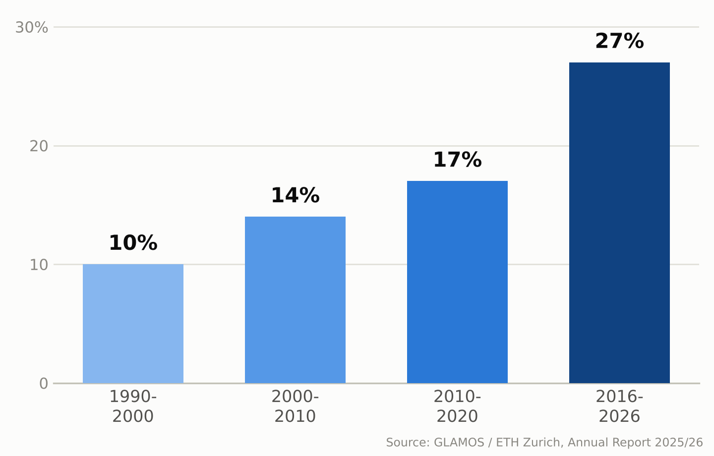
    Zoom out and the five-year picture is starker. Since 2021, Swiss glaciers have lost close to 20% of their remaining volume — a loss rate GLAMOS describes as more than twice as fast as any earlier five-year period in its record. The longer-term picture shows the same acceleration: Swiss glaciers lost about 10% of their volume in 1990–2000, 14% in 2000–2010, 17% in 2010–2020, and about 27% over the most recent ten-year window, 2016–2026.

    Bar chart showing Swiss glacier ice volume loss by decade: 10% in the 1990s, 14% in the 2000s, 17% in the 2010s, and 27% in 2016-2026
    Share of ice volume lost by Swiss glaciers, by decade. Source: GLAMOS / ETH Zurich, Annual Report 2025/26.

    Why this past year was so bad

    Two seasons combined to make 2025/2026 so damaging. Winter snowfall came in about 25% below the long-term average by the end of April, leaving glaciers with a thin protective layer heading into summer. The following April–September period was, according to glaciologist Matthias Huss, who leads GLAMOS and is a professor at ETH Zurich, the hottest and driest “summer half-year” in Switzerland since national weather records began in 1864. The freezing level — the altitude of the 0°C mark in the atmosphere — rose above 4,000 meters on 76 days, more than double the average and a new Swiss record. By September, snow cover had disappeared even at elevations around 3,500 meters.

    GLAMOS calls the point when melt overtakes the winter’s snow gains — after which every melted liter comes straight out of the glacier’s mass — “Glacier Loss Day.” In 2026 that point arrived on June 29, the second-earliest date on record, three days later than the record set in 2022. One reason 2026 still fell just short of 2022’s record was the smaller amount of Saharan dust deposited on the snow that year, which let glaciers reflect more sunlight than they did in 2022, when dust darkened the surface and accelerated melting.

    Melting is also carving cavities and collapse zones into some glaciers

    Researchers monitoring the retreat describe an additional process layering on top of ordinary surface melting. On some glacier tongues, meltwater penetrates and flows through the ice, forming channels and cavities; where these grow large enough, sections of ice can collapse inward rather than simply retreating at the edges. Huss has described visiting high-altitude sites that were still covered in ice a few years ago — including areas near the Grosser Aletsch’s Konkordiaplatz and around the Findel glacier by the Matterhorn — and finding bare, rubble-strewn rock he compared to a lunar landscape.

    Some glaciers are also disappearing outright. The Bella Tola glacier in canton Valais, which had been measured for decades, is among the small glaciers researchers now consider completely and permanently gone as of 2026. GLAMOS estimates that roughly another 100 small Swiss glaciers disappeared between 2016 and 2023 — a pace this year’s melt appears to be extending rather than slowing.

    A record summer of meltwater is also a warning sign

    Between July and September 2026 alone, Swiss glaciers released an estimated 2.2 trillion liters of water — more than four times the amount all Swiss households drink in a year.

    Between July and September 2026, Swiss glaciers released roughly 2.2 trillion liters of meltwater — equivalent to more than four times the annual drinking-water consumption of every household in Switzerland.

    That sounds like abundance, and in the short term it was: the extra runoff topped up rivers during a hot, dry summer when demand for water was high. But glaciologists are blunt about what it really represents — a one-time withdrawal from a shrinking reserve, not a renewable supply. Glaciers act as a buffer that releases extra meltwater precisely in hot, dry years when it’s needed most; snowfall can replenish that mass over time, but only when accumulation exceeds losses, which has not been the case in most recent years. As the ice reserve keeps shrinking, its ability to smooth out future droughts shrinks with it.

    That matters beyond Switzerland too. Glacier melt contributes to summer runoff in Alpine river basins, including the Rhône and the Rhine, helping sustain flows during hot, dry periods for communities downstream in France, Germany, and beyond. The 2026 season offered unusually generous meltwater precisely because the ice had so much to give up. A smaller, thinner body of Alpine glaciers will have less stored ice to release in the next hot summer, and some smaller glaciers may disappear entirely.

    What the long record shows

    GLAMOS’s value lies partly in its length: continuous measurements stretching back decades let scientists tell a single rough year apart from a structural shift, and the longer-term record shows increasingly rapid losses, with the most recent ten-year period (2016–2026) substantially exceeding the losses seen in each earlier ten-year period. By the end of the 2025/2026 measurement season, Switzerland’s glaciers held an estimated 42.6 cubic kilometers of ice across 714 square kilometers of glacier-covered area — down by more than 30 cubic kilometers, and about a third in glacier-covered area, since 2000.

    Researchers caution against reading any single year, including 2026’s near-record losses, as proof of exactly what comes next; Alpine weather still varies year to year, and a cold, snowy winter can briefly slow the trend. But the multi-decade pattern GLAMOS has documented — each ten-year period worse than the last — is increasingly relevant to how water-resource managers, hydropower operators, and mountain communities across the Alps plan around the region’s future water supply.

    Sources: ETH Zurich, “Devastating year for Switzerland’s glaciers”, GLAMOS, Annual Report on Swiss Glaciers 2025/26, PBS NewsHour / Associated Press

  • [Science] The Instant You Decide, Your Brain Re-Files the Options — MIT Neuroscientists Find a Flexible Code That Could Inform AI Design

    [Science] The Instant You Decide, Your Brain Re-Files the Options — MIT Neuroscientists Find a Flexible Code That Could Inform AI Design

    Every time you choose between two options — which job offer to accept, which product to buy — your brain does more than simply retrieve what each one was worth. A new MIT study shows that the instant you make that choice, the neural code representing those options in part of your brain reorganizes itself, shifting from grouping information by the order you saw it to grouping it by whether you picked it. The finding, published online in the journal iScience in September 2026, offers a rare, cell-by-cell look at how flexible biological memory can be — and it gives researchers working on adaptive AI a biological case study worth studying, even though the experiment itself did not involve any AI system.

    Why Scientists Wanted to Watch the Brain Mid-Decision

    Researchers have long known that the prefrontal cortex, the region of the brain just behind the forehead, plays a central role in weighing options and making choices. Many of its neurons also show “mixed selectivity,” meaning a single cell’s activity can shift depending on a combination of task variables rather than tracking one fixed thing. What earlier work left unresolved was how the brain avoids mixing up two options that were evaluated only moments apart, especially once one has been chosen and the other set aside. A team led by MIT graduate student Huidi Li and senior author Earl K. Miller, a professor at MIT’s Picower Institute for Learning and Memory, set out to track that process neuron by neuron rather than assume an answer. The team, which also included Nikolaos Chrysanthidis, Scott Brincat, and Jonas Rose, published its results in iScience; MIT publicized the findings on September 22.

    Watching Hundreds of Neurons Decide, in Real Time

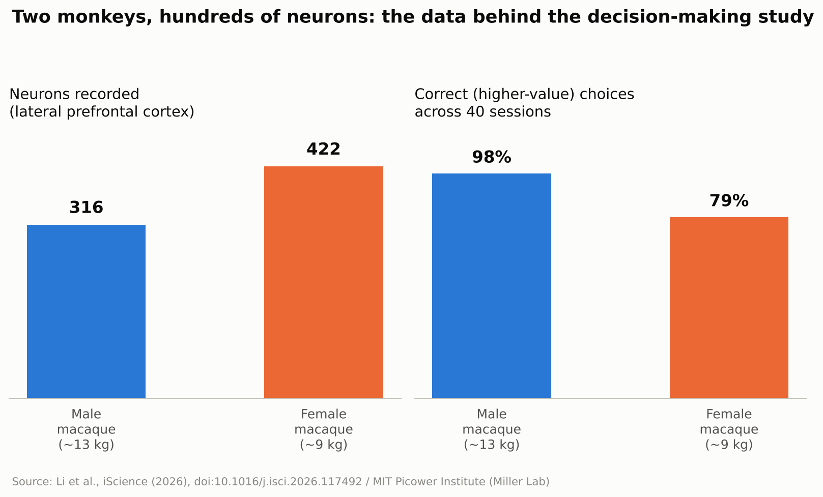
    To find out, the researchers trained two macaque monkeys — a roughly 13-kilogram male and a 9-kilogram female — to play a simple reward game. A white square flashed briefly at one of four spots on a screen, followed by a colored ring that signaled how many drops of juice that option was worth, anywhere from one to thirteen. The same sequence then repeated for a second target at a different screen location. Once both options had been shown, the monkey looked toward its preferred target and received the corresponding juice reward. The male selected the higher-value option on about 98 percent of trials; the female, on about 79 percent. While the animals made their choices, the team recorded the electrical activity of 316 neurons in the male’s lateral prefrontal cortex — the side portion of the prefrontal cortex — and 422 in the female’s, across 40 recording sessions. Rather than tracking single cells in isolation, the researchers analyzed the activity of the whole recorded population as points moving through a high-dimensional mathematical space, a technique known as neural subspace analysis: when enough neurons fire in a similar combined pattern, that pattern occupies its own region, or “subspace,” within that space, and two subspaces that barely overlap are described as close to orthogonal, or mathematically independent of each other.

    Bar chart showing neurons recorded and choice accuracy for two macaques in the study
    Source: Created from data in Li et al., iScience (2026)

    Before the Choice: Order. After the Choice: Outcome.

    Seen through that lens, the result is a clear shift in organization. Before a choice was made, the subspaces representing the first-shown and second-shown targets were kept largely separate, organized around presentation order. Once the monkey chose, the picture changed: the subspaces reorganized around the decision itself, with the chosen and unchosen options rotating into distinct, close-to-orthogonal subspaces regardless of the order in which they had originally appeared. In other words, the brain’s filing system for “what I saw first and second” gave way to a new one built around “what I picked and what I didn’t.” The researchers suggest this reorganization helps downstream brain regions read out the decision efficiently, since they could rely on a consistent format rather than track which position each option had occupied.

    “The brain doesn’t just hold information statically,” Li said.

    No Single Neuron “Owns” a Decision

    A second notable result was how that reorganization happened at the level of individual cells. The researchers found no fixed set of neurons permanently dedicated to representing “the chosen option” or “the rejected one.” Instead, individual neurons shifted which ensemble they contributed to from one trial to the next, joining a different, temporary coalition of cells depending on what the task required at that moment. Researchers in the field generally see this kind of flexible, overlapping coding as a way for a limited number of neurons to represent many different combinations of information, rather than requiring a dedicated cell type for every possible scenario — though this study did not directly measure how much representational capacity that flexibility adds.

    Why This Matters Beyond the Lab

    The study did not test any artificial intelligence system, and the researchers were not trying to build one. Still, the result speaks to a question AI researchers care about: how can a learning system keep updating what it represents without losing track of information it already holds? Many AI systems, once trained, represent what they have learned in ways that stay largely fixed afterward, which is part of why training them further on new material can degrade old knowledge, a problem researchers call catastrophic forgetting. The MIT findings do not explain or solve that problem, but the underlying idea — a biological circuit reorganizing its internal representations on the fly to match what a task demands at each stage — is the kind of mechanism that researchers in continual learning and brain-inspired, or neuromorphic, computing study for design ideas. It is also a small, concrete answer to a more everyday question: the researchers found that even after a choice was made, the unchosen option remained represented in its own distinct subspace rather than disappearing from the recorded activity. MIT’s own description of the work suggested this could be important for later crediting an outcome to the option that produced it, which may help the brain learn from an alternative it did not select — though that specific learning process was not directly tested in this experiment.

    What’s Still Unknown

    The authors are careful to flag the limits of the work. Only two animals took part, and the task involved a simple, sequential choice between two options with clearly different, discrete reward values — closer to comparing two job offers one after the other than to scanning a crowded menu of possibilities at once. Whether the same kind of reorganization occurs when values vary continuously, when there are more than two options on the table, or in human decision-making specifically, remains an open question the team says future studies will need to address. Macaque and human prefrontal cortex share many organizational similarities, which is why monkey studies like this one are routinely used to generate hypotheses about human cognition, but confirming that the same reorganization happens in people would require a separate study in humans. It is also worth remembering that this was a recording study: it shows that representations change alongside decisions, not that the reorganization itself is what causes a choice to happen. As with any single study, independent replication will matter before the finding is considered settled.

    For now, the study offers a concrete, carefully measured answer to a question that sounds almost philosophical: what happens in your head in the instant after you decide? According to this research, at least in one brain region of two monkeys performing a simple task, the answer is that the brain quietly rebuilds how it was organizing two competing options around the choice that was just made.

    Sources: MIT News, iScience (Li et al., 2026), EurekAlert!

  • [Science] The Ice Shooting Off Saturn’s Moon Enceladus Isn’t a Simple Copy of Its Ocean — A Finding That Could Reshape the Hunt for Alien Life

    Every second, the icy moon Enceladus sprays countless grains of ice from its hidden ocean into space, feeding one of Saturn’s rings. An international team led by the Freie Universität Berlin and the Earth-Life Science Institute at the Institute of Science Tokyo has proposed that, on the way out, that water gets chemically sorted. The upshot: an individual ice grain is not simply a miniature sample of the whole ocean, which matters for any future mission trying to read Enceladus’s ocean chemistry for signs of life.

    Original source
    Journal: Science Advances (DOI: 10.1126/sciadv.aee7256)
    Press release: Freie Universität Berlin
    Data: 961 ice-grain spectra recorded by Cassini’s Cosmic Dust Analyzer

    Cooling speed decides which salt goes where

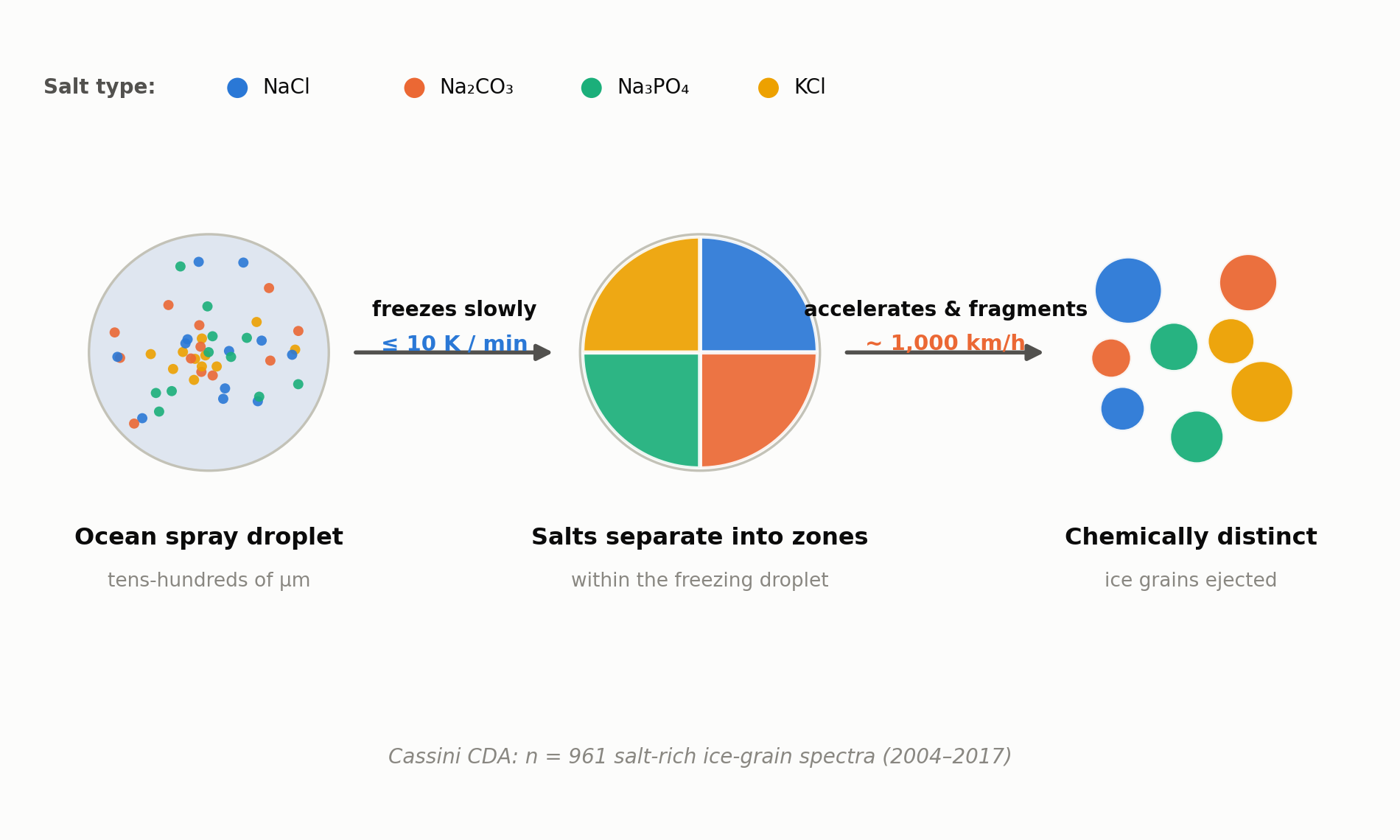
    The team ran lab experiments with droplets formulated to match the salts expected in Enceladus’s subsurface ocean. When droplets roughly 200 micrometers across were cooled slowly, at about 10 kelvin per minute or less, the dissolved salts did not freeze evenly into the ice. Instead, compounds such as sodium chloride, carbonates, phosphates and potassium salts separated out and concentrated into distinct regions within the droplet as it froze. Rapid freezing did not produce the same pronounced separation, the experiments showed.

    961 oddly different ice grains from Cassini

    What happens to a droplet after it freezes unevenly underground? The team proposes that as these droplets rise through narrow vent channels toward the surface, they accelerate — reaching roughly 1,000 km/h in the model — before shattering against the icy channel walls into the fine grains that eventually reach space. NASA’s Cassini spacecraft, which orbited Saturn from 2004 to 2017, carried a Cosmic Dust Analyzer (CDA) that recorded mass spectra for 961 salt-rich ice grains gathered over the course of its mission. Grain to grain, the chemistry varied widely — some grains dominated by sodium salts, others by carbonates or phosphates — even though they presumably all came from the same ocean. The new freeze-and-fragment model offers an explanation for why that is: each grain simply froze out of a different, already-segregated pocket of the original droplet.

    “The oceanic constituents are separated from each other and simultaneously concentrated into individual ice particles,” says Professor Frank Postberg of Freie Universität Berlin.
    Schematic of the proposed ice-grain formation model at Enceladus
    Source: created from data released by Freie Universität Berlin / Institute of Science Tokyo (proposed grain-formation model)

    A discovery that could change how we read the data

    The core implication is that no single ice grain can be assumed to represent the ocean’s average composition. That matters for mission concepts such as NASA’s proposed Orbilander, which would collect and analyze Enceladus’s plume grains directly: researchers will likely need to account for grain-to-grain differences when interpreting what they find. The team suspects organic molecules and other life-relevant compounds could be concentrated in a similar way, though confirming that will require further study.

    Enceladus remains one of the solar system’s most closely watched candidates for hosting life. Understanding how each ice grain came to be — rather than treating it as a simple drop of seawater — looks set to become an unavoidable consideration for the missions that follow.

    Xsciens editorial note

    This study is a model that explains an existing dataset, not a new observation of Enceladus. Its central claim, that cooling speed determines which salts end up in which ice grains, is a proposal that fits the 961 Cassini spectra. It has not been confirmed by a new spacecraft measurement. The reading is attractive because it ties grain composition to a physical process, but it also means any future mission, such as the Orbilander concept, would need to test it directly before the interpretation of the data is changed.

    Key terms

    • Cosmic Dust Analyzer (CDA): the Cassini instrument that analyzed the composition of individual ice grains in flight.
    • Cooling rate: how fast a droplet loses heat; the study ties it to which salts crystallize in a grain.
    • Vent: a fissure on Enceladus’ south pole through which water-rich material is ejected into space.

    Sources: Freie Universität Berlin press release, Science Advances (DOI: 10.1126/sciadv.aee7256)