Author: Y. Y.

  • [Science] Forest Lizards Gained About 2°C of Heat Tolerance in a Decade

    [Science] Forest Lizards Gained About 2°C of Heat Tolerance in a Decade

    Lizards living deep in Caribbean forests can now tolerate about 2°C more heat than their counterparts a decade ago, while species that can step into cooler spots barely changed. The contrast, reported by a Yale-led team in PNAS, suggests that an animal’s habitat and its ability to regulate body temperature through behavior may influence how quickly its heat tolerance changes in a warming world.

    原論文情報 / Original Paper
    Title: “Thermal ecology drives alternate responses to rising temperatures in Caribbean anoles”
    Authors: Saúl F. Domínguez-Guerrero et al.
    Journal: Proceedings of the National Academy of Sciences (2026)
    DOI: 10.1073/pnas.2537152123

    What the team found

    Researchers led by Saúl Domínguez-Guerrero and Martha Muñoz at Yale University compared how well 16 species of Caribbean anoles, small tree-dwelling lizards, handle extreme heat. The species live on three islands: Hispaniola, Jamaica and Puerto Rico.

    The team did not set out to catch evolution in action. They were studying how behavior shapes physiology, and they expected familiar results. Back in New Haven, though, the temperature data told an unexpected story, and a colleague’s offhand remark that something looked “weird” turned into the paper.

    The measure at the center of the study is the critical thermal maximum, or CTmax: roughly, the highest body temperature an animal can tolerate before reaching a defined point of impairment in an experiment. It is a measured threshold, not a prediction of the temperature that would kill the animal. Earlier teams had measured it for the same group of species on the same islands in 2011–2013. The Yale team repeated the work in 2022–2025, giving them a before-and-after comparison across roughly a decade.

    Not every species moved the same way

    The surprise was that the shifts were not uniform. Species in open or forest-edge habitats showed little change in heat tolerance. These lizards can move into shade or onto cooler perches, which helps keep their body temperatures in a suitable range. This strategy is known as behavioral thermoregulation.

    Species deep in closed forest canopy told a different story. With far fewer ways to escape the heat, their heat tolerance rose by about 2°C over the decade. According to the researchers, thermal ecology, meaning how an animal navigates the temperatures available in its environment, predicted these changes better than evolutionary relatedness or geographic closeness did.
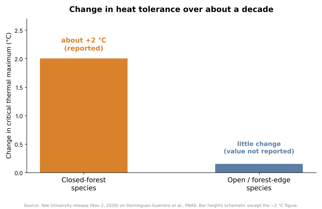
    Bar chart: closed-forest anoles gained about 2 degrees C of heat tolerance in a decade, open-habitat species changed little
    Figure 1. Reported change in heat tolerance over about a decade. Only the ~2 °C figure is a reported value; the other bar is schematic. Source: Yale University release on Domínguez-Guerrero et al., PNAS (2026).

    Why habitat matters

    An animal that can move into cooler surroundings may reduce its exposure to extreme heat, which lessens the pressure on its body to become more heat-tolerant. But when cooler places are scarce or hard to reach, the animal has fewer ways to avoid overheating, and stronger pressure for physiological change may follow. In the researchers’ words, behavior may help determine not only how animals respond to environmental change, but also how quickly they evolve.
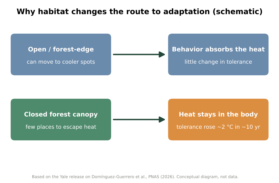
    Schematic: open habitats let lizards use behavior to avoid heat, closed forest leaves heat on the body and tolerance rose
    Figure 2. Conceptual diagram of the two routes (not measured data). Source: based on the Yale University release.

    Behavior as a buffer and a brake

    This logic echoes older work. In a 2003 paper in The American Naturalist, Raymond Huey and colleagues described how thermoregulatory behavior can reduce the selection pressure for changes in thermal physiology, an effect they called the Bogert effect. A 2014 PNAS study led by Jennifer Sunday, covering 296 species of cold-blooded animals, found that heat-tolerance limits are broadly similar across latitude and elevation, that tropical species lean more on behavior such as seeking shade, and that few species have much spare heat tolerance.

    Against that background, the Yale study adds a before-and-after comparison, over a decade, of closely related lizards that differ in their opportunities for behavioral thermoregulation.

    The team also tested lizard offspring to see whether the higher heat tolerance can be inherited. The Yale release does not detail the outcome, so readers who want the answer should consult the paper itself. In follow-up work mentioned by the researchers, similar patterns appear in lizard populations in Mexico, and frog tadpoles in temperature-stable ponds also seem to be gaining heat tolerance. Those observations were described only briefly.

    Not an escape hatch

    Lead author Domínguez-Guerrero cautions that both behavioral and physiological responses have limits. “These lizards may be racing to keep up,” he said, but they may eventually hit an “evolutionary ceiling,” a point beyond which their bodies can no longer adapt. The study did not establish where such a ceiling lies; the term is the researcher’s warning rather than a measured result.

    Rapid increases in heat tolerance in some species do not mean climate warming is harmless for reptiles. They show that different species respond in different ways, and that some may be better placed to cope than others.

    Xsciens Editorial Note

    Core point: lizards that cannot escape heat gained about 2°C of heat tolerance in ten years, while species with cooler hiding places changed little.

    • Observation versus interpretation. What was measured is the upper heat limit of 16 species at two points in time, 2011–2013 and 2022–2025. A before-and-after comparison alone cannot separate genetic evolution from flexible adjustment within an animal’s lifetime, so calling the change “adaptation” is the researchers’ interpretation. The roughly 2°C figure is for closed-forest species as a group, not every species.
    • Limits. The study compares two measurement periods rather than tracking the lizards continuously, and covers 16 species on three islands, so the pattern may not hold for all animals. We worked from the university release and news coverage because the full paper was not accessible to us, so details such as sample sizes per species were not available. The Mexico lizard and tadpole findings were mentioned only briefly.
    • What to watch next. How much of the change is heritable, whether other regions and animal groups show the same split, and how far heat tolerance can rise before physiological limits are reached. The 2014 survey of 296 species found few with much spare heat tolerance.
    • From the editors — a shady patch of forest may be worth as much to wildlife as any technological fix. If the pattern holds, planners could use it to spot species with few cool places to retreat to and protect the shade, dense vegetation and cool refuges around them first, though this study did not test such measures. The warning is built in: the researchers themselves expect an upper limit, so this is no reason to relax about warming. For the rest of us, even a tree, some shade and a water dish in a backyard count as habitat for the small animals nearby.

    References for this note: Huey, Hertz & Sinervo (2003), The American Naturalist, Sunday et al. (2014), PNAS

    Sources: Yale News, Phys.org, PNAS (Domínguez-Guerrero et al., 2026)
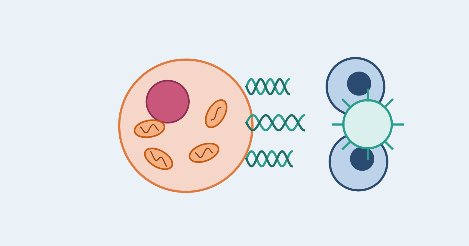
  • [Science] Mitochondrial DNA May Decide Whether Dying Cancer Cells Alert the Immune System

    [Science] Mitochondrial DNA May Decide Whether Dying Cancer Cells Alert the Immune System

    Whether a dying cancer cell wakes up the immune system may depend on how much mitochondrial DNA it carries. A Japanese research team reports that cancer cells carrying KRAS mutations tend to accumulate mitochondrial DNA, and that a combination of drugs can make such cells die in a way that alerts the immune system. So far this has been shown only in cell experiments and mice, not in patients.

    原論文情報 / Original Paper
    Title: Mitochondrial DNA abundance is a determinant of immunogenic cell death in cancer
    Authors: Kosuke Tanaka, Yasuki Adachi, et al.
    Journal: Immunity (2026)
    DOI: 10.1016/j.immuni.2026.10.002

    Why the way a cancer cell dies matters

    Many cancer drugs work by killing tumor cells, but cells can die in different ways. In apoptosis, an orderly form of cell death, dead cells are generally cleared away without a strong immune response. Some deaths, however, alert the immune system. Researchers call this immunogenic cell death: the dying cells release signals that help immune cells recognize tumor material and go after surviving cancer cells. A widely cited 2020 consensus paper describes it as death that provides enough “antigenicity and adjuvanticity”, roughly, enough recognizable tumor antigens and enough additional signals to activate an immune response.

    This matters for treatment. Targeted drugs that block a specific faulty molecule in a tumor often work well at first, but cancers can resist them or relapse. Pairing them with immune checkpoint inhibitors, drugs that release the brakes on immune cells, is an attractive idea. Whether the pairing works may depend on whether the targeted drug makes cancer cells die in a way the immune system can see, and what decides that has been poorly understood. The researchers therefore asked whether something inside the cancer cell itself could tip the balance. Their attention turned to mitochondria, the structures that produce energy for the cell.

    KRAS-mutant cancers hoard mitochondrial DNA

    Mitochondria carry a small loop of their own DNA, called mtDNA. When mtDNA leaks into the main body of the cell, a protein called cGAS detects it and activates another protein, STING. This cGAS-STING pathway triggers the production of type I interferons, immune signaling proteins that help alert the body’s defenses.

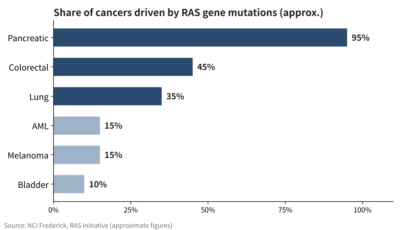
    The team first mined public databases of cancer cell lines. Whether a line carried a KRAS mutation tracked its mtDNA level more closely than the type of cancer did, and lung, colorectal, pancreatic and biliary cancers with KRAS mutations tended to hold more mtDNA. According to the researchers, KRAS mutations increase reactive oxygen species (ROS), chemically reactive molecules that can damage cell components, and these also promote the copying of mtDNA. Such cancers are common: the U.S. National Cancer Institute’s RAS Initiative estimates that mutations in the RAS gene family, which includes KRAS, are found in roughly a third of human cancers, including about 95 percent of pancreatic cancers, 45 percent of colorectal cancers and 35 percent of lung cancers.

    Bar chart of approximate shares of cancers with RAS gene mutations: pancreatic 95%, colorectal 45%, lung 35%, AML 15%, melanoma 15%, bladder 10%
    Source: NCI Frederick, RAS Initiative (approximate figures). RAS is the gene family that includes KRAS.

    Letting the DNA out, then removing the brake

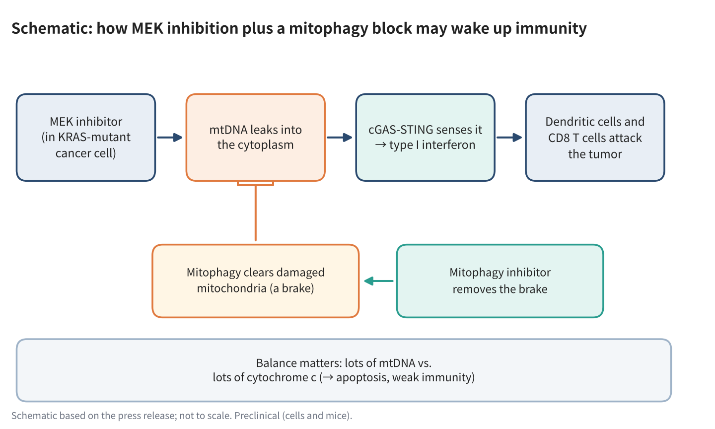
    In KRAS-mutant cells, a drug that blocks MEK, a protein in the same growth-signaling chain as KRAS, made mtDNA escape into the cytoplasm. But the drug also switched on mitophagy, the cell’s routine for clearing out damaged mitochondria, which limited the leak. The team found that this cleanup involved a protein called PRKN, which helps remove damaged mitochondria and thereby holds back the release of mtDNA.

    The two drugs thus work in opposite ways: one causes mitochondrial damage and releases mtDNA, while the other stops the cell from cleaning up. When the researchers added chloroquine, which they used experimentally to inhibit mitophagy, damaged mitochondria were no longer cleared as effectively, mtDNA kept escaping, and the type I interferon response grew stronger. The response did not appear in cells with little mtDNA or in cells lacking STING. Across human cancers, the team also noted that higher PRKN expression went along with less immune-cell infiltration.

    Schematic of MEK inhibition plus a mitophagy block causing mtDNA leakage, cGAS-STING signaling and an immune attack on the tumor
    Schematic based on the press release; not to scale. Preclinical (cells and mice).

    A balance with cytochrome c

    There was a second ingredient. Cytochrome c is a protein normally involved in energy production inside mitochondria; when released into the cell, it helps trigger the machinery of apoptosis. The researchers found that the relative amounts of mtDNA and cytochrome c help determine whether drug-treated cells undergo apoptosis or immunogenic cell death.

    In lung cancer cells with a lot of mtDNA, such as those with KRAS mutations or ALK or ROS1 gene fusions, the drug combination produced an immune response. In EGFR-mutant lung cancer cells, which carry a lot of cytochrome c, cells mainly died by apoptosis, and lowering cytochrome c shifted them toward immunogenic death. Pushing the drugs too hard also favored apoptosis and weakened the immune response, a hint that simply killing more cancer cells is not always the better goal.

    What happened in mice

    In a mouse model of KRAS-mutant colorectal cancer, the team combined a MEK inhibitor, a mitophagy inhibitor and an anti-PD-1 antibody, a type of checkpoint inhibitor. The three-drug combination suppressed tumor growth, and tumors disappeared in 2 of 12 mice. The effect depended on dendritic cells, which show tumor fragments to other immune cells, and on CD8-positive T cells, the immune system’s cancer-killing cells. Tumors with low mtDNA did not respond. These results show an effect in a preclinical model; whether the same strategy can work in patients remains unknown.

    The findings suggest that successful cancer treatment may depend not only on how many cancer cells are killed, but also on how their deaths affect the immune system. According to the press release, the team’s next steps are to test whether mtDNA abundance can predict how patients respond to treatment and to develop strategies that combine targeted drugs with immunotherapy. The work was supported in part by Japan’s AMED and the Moonshot R&D Program.

    Xsciens Editorial Note

    The study suggests that how much mitochondrial DNA a tumor carries helps decide whether drug-induced cell death rouses the immune system.

    • Observation versus model. What was observed: KRAS mutation tracked mtDNA levels in public cell-line data, and the drug combination caused mtDNA leakage and interferon signaling in cells. The mtDNA-versus-cytochrome c “balance” is the team’s explanation, built from experiments in which those molecules were manipulated in cells. The 2-of-12 figure counts complete tumor disappearance in mice, not an overall response rate.
    • Limits. The evidence comes from cell experiments, analyses of public cancer databases and mouse models. Although the researchers looked at patterns in human cancers, they have not shown that the drug combination works in patients. Chloroquine was an experimental tool to inhibit mitophagy, not a validated cancer treatment, and nothing here supports anyone taking it for cancer.
    • What to watch. Whether mtDNA abundance can predict treatment response in patients, and whether it must be read alongside cytochrome c levels and other features of the tumor environment. The team says this still needs testing.
    • From the editors — if this holds up, cancer care could get smarter about how tumors die, not just whether they do. Doctors might one day check a tumor’s mitochondrial DNA to pick drugs that leave the immune system alert to any survivors, which could mean fewer relapses. But all of this rests on cells and mice so far, and pushing a tumor too hard can backfire, as this very study shows. If you or someone close is in treatment, keep an eye on this field, but treat no single drug as the answer.

    References for this note: Galluzzi et al., Consensus guidelines for the definition, detection and interpretation of immunogenic cell death (J Immunother Cancer, 2020), NCI Frederick, RAS Initiative, Lin et al., Editorial: Mitochondrial damage interacts with the immune system and tumor microenvironment (Front Immunol, 2025)

    Sources: Immunity (Tanaka et al., 2026), Nagoya University / National Cancer Center Japan / Kyoto University press release (Nov 2, 2026, in Japanese), Kyoto University research news (in Japanese)

  • [Science] Possible New Dwarf Planet Beyond Pluto Found in Rubin Observatory Data

    [Science] Possible New Dwarf Planet Beyond Pluto Found in Rubin Observatory Data

    Astronomers using data from the Vera C. Rubin Observatory have identified an object called 2026 ED138, currently about 46 times farther from the Sun than Earth is and perhaps 600 to 1,500 kilometers across — large enough that it may qualify as the solar system’s sixth dwarf planet. It matters because it shows that sizable worlds can still hide in the outer solar system, and that new survey data and search software are now able to dig them out.

    原論文情報 / Original Paper
    Announcement: Possible new dwarf planet 2026 ED138 (provisional designation)
    Announced by: NSF–DOE Vera C. Rubin Observatory / NOIRLab, October 27, 2026
    Discoverer: Matthew Holman, Center for Astrophysics | Harvard & Smithsonian
    Peer-reviewed paper: none cited in the coverage we checked. Source: University of Washington News

    What the team found

    The object carries the provisional name 2026 ED138. It was first identified on the evening of October 13, 2026, by astronomer Matthew Holman of the Center for Astrophysics | Harvard & Smithsonian, who was sifting through images that the NSF–DOE Vera C. Rubin Observatory had collected earlier this year; the University of Washington describes that data as preliminary. The object had been photographed before, but never recognized as a single moving body. Holman developed the search code together with colleague Kevin Napier. It links billions of detections of moving objects to work out which ones belong to the same body. Holman has described his first reaction as “excited disbelief,” and he immediately checked whether he or the code had made a mistake.

    Once the candidate was in hand, more data fell into place. According to Space.com and Universe Today, Rubin’s telescope recorded it 30 times on 20 nights between March 4 and July 11, 2026. Mario Jurić of the University of Washington, who leads Rubin’s solar system team, turned up additional detections in the catalog. Archival images from other surveys, including the Dark Energy Camera on a 4-meter telescope in Chile, extend the record back to 2016. That gives the team more than a decade of positions from which to calculate the orbit.

    Where it was hiding

    ED138 is currently about 46 astronomical units from the Sun (one astronomical unit is the Earth–Sun distance), compared with about 40 for Pluto on average. Its orbit is tilted roughly 25 degrees from the plane in which the planets travel, a tilt Space.com says likely stems from a gravitational interaction with Neptune. Universe Today describes it as a “hot classical” object, a label for icy Kuiper belt bodies on more tilted, disturbed orbits.

    The location also helps explain why it was missed. ED138 lies in a region near the plane of our own galaxy, where the Milky Way’s dense star field makes faint, slowly moving dots hard to pick out. The University of Washington’s write-up says this likely hid it from most other telescopes. Finding it took both Rubin’s repeated imaging and software built to link scattered faint detections. We covered a similar story of patient, data-driven discovery in our earlier piece on a possible hidden pair of supermassive black holes.

    How big is it, really?

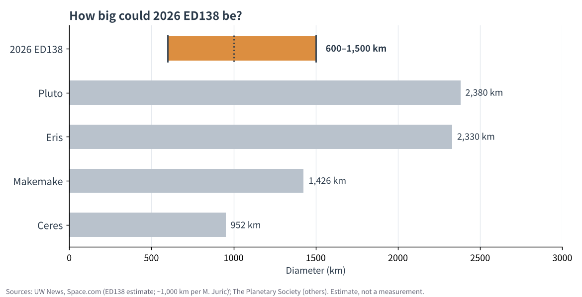
    The headline estimate is 600 to 1,500 kilometers across. That would put ED138 anywhere from a modest icy world, smaller than Ceres, up to one comparable to the dwarf planet Makemake, which is about 1,430 km wide according to The Planetary Society. Jurić has put the best guess near 1,000 km and, as Gizmodo reports, called it the largest trans-Neptunian object found in about 20 years. Those figures remain estimates.

    Bar chart comparing the estimated 600 to 1,500 km size of 2026 ED138 with Ceres, Makemake, Eris and Pluto
    Estimated size of 2026 ED138 compared with known dwarf planets. Sources: UW News, Space.com, Gizmodo (ED138 estimate); The Planetary Society (others).

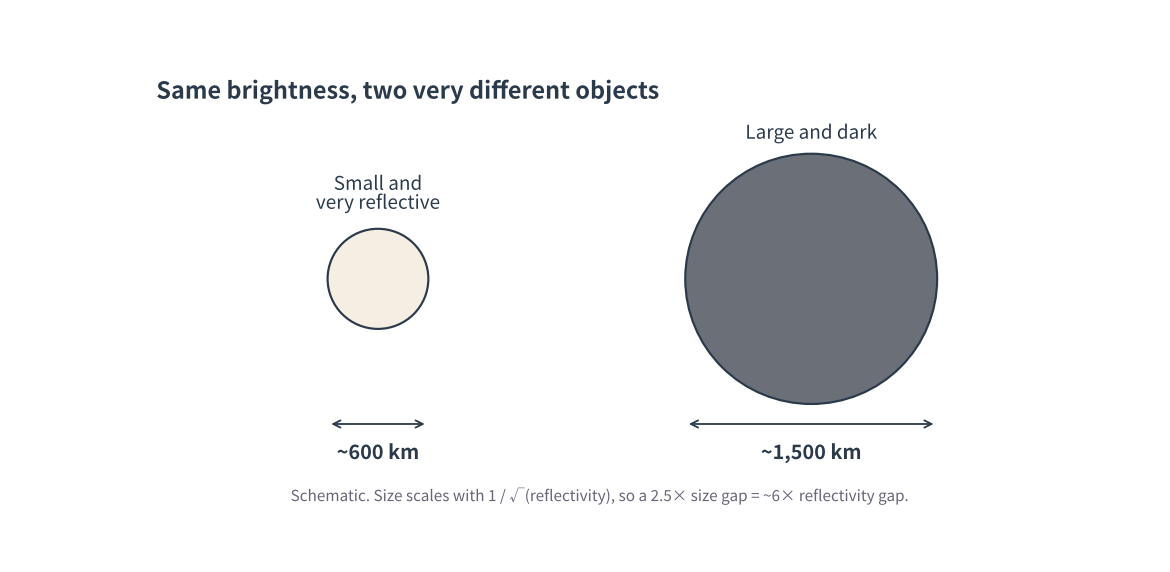
    Why such a wide range? Telescopes see reflected sunlight, and how much light arrives depends on two things at once: how big the object is and how reflective its surface is (its albedo). A small, shiny body and a large, dark body can look equally bright from far away. The team estimated size from distance, brightness and an assumed surface reflectivity, so the range mostly reflects uncertainty about that reflectivity. A 2.5-fold gap in diameter corresponds to roughly a six-fold gap in albedo.

    Schematic of a small reflective body and a large dark body appearing equally bright
    Schematic: the same brightness can come from a small, reflective object or a large, dark one. Created by Xsciens.

    What counts as a dwarf planet

    NASA summarizes the International Astronomical Union’s definition: a dwarf planet orbits the Sun, is massive enough for its own gravity to pull it into a nearly round shape, has not cleared the neighborhood around its orbit, and is not a moon. Five objects are recognized today: Ceres, Pluto, Eris, Haumea and Makemake. If ED138 is confirmed to meet the criteria and is formally recognized, it would be the sixth.

    Roundness is why size matters so much. The University of Washington’s write-up notes that icy bodies of this scale are expected to be round, but nobody has yet observed ED138 well enough to see its shape. Until its diameter and shape are measured, “candidate” is the accurate word.

    What happens next

    Follow-up work will aim to pin down the size. Space.com reports that this requires infrared observations, naming the James Webb Space Telescope, because an object’s heat emission helps separate its size from its reflectivity. Meanwhile, Rubin’s ten-year survey of the southern sky, which began in June 2026, continues, and searches of older images — “precovery,” in Jurić’s term, meaning finding an object in images taken before anyone recognized it — may turn up more objects earlier surveys missed.

    In the coverage we checked, no peer-reviewed paper accompanies the announcement, so the numbers above should be read as the team’s preliminary estimates.

    Xsciens Editorial Note

    This is a candidate, not a confirmed dwarf planet: its orbit is calculated from about a decade of positions, but its size is still an estimate.

    • Observed versus calculated. What astronomers recorded directly were positions and brightness in many images. The distance (about 46 au) and the orbital tilt (about 25°) are calculated from them, and the 600–1,500 km diameter is a further estimate that also assumes how reflective the surface is, which is why the range spans a factor of 2.5.
    • Limits. Roundness has not been observed, and the coverage we reviewed cites no peer-reviewed paper. This note rests on the announcement and secondary coverage; we could not open the NOIRLab release itself. “Hot classical” is Universe Today’s description, for a category of Kuiper belt objects defined by widely tilted orbits.
    • What to watch. Infrared measurements of its size, for which Space.com points to the James Webb Space Telescope, and whether the object is formally recognized as a dwarf planet.
    • From the editors — the solar-system poster on a classroom wall may soon need a new line. If Rubin keeps scanning the southern sky for ten years, more faint worlds could plausibly turn up, ones that hid in crowded star fields or slipped between older surveys. The catch is that “candidate” is the operative word, and until the size is measured the headline number could move a lot. So treat 1,000 km as a placeholder, and look again when the infrared measurements arrive.

    References for this note: NASA, What is a planet?, Müller et al., Trans-Neptunian objects and Centaurs at thermal wavelengths (arXiv), Petit et al., Canada-France Ecliptic Plane Survey (arXiv)

    Sources: University of Washington News, Space.com, Universe Today, Gizmodo, The Planetary Society

  • [Science] Why Is Japan So Strong in Materials? The Industry Structure and Three Hypotheses, Read Through Cases

    [Science] Why Is Japan So Strong in Materials? The Industry Structure and Three Hypotheses, Read Through Cases

    The chips in a smartphone, the airframe of a jet and the battery in an electric car all get their performance from materials. In materials, Japanese companies hold a majority of world share in a number of fields. This article checks the current picture and the challenges against official documents, lays out the industry structure materials sit in, and then digs into why Japan is strong through three hypotheses and company cases.

    Key data in this article
    • METI, New Materials Industry Vision (interim summary, June 2022): Materials are 20% of manufacturing GDP; Japanese firms hold 70% of photoresist, and one firm (Company A) 80% of rolled copper foil for FPCs
    • METI, Global Niche Top Companies 100 (2020 edition): 113 selected firms: average world share 43.4%, average operating margin 12.7% (manufacturing average 4.8%)
    • Cabinet Office, Materials Innovation Strategy (June 2025): Many materials above 60% world share; names “suriawase-type development” as a Japanese strength

    Where things stand: strength in share and margins

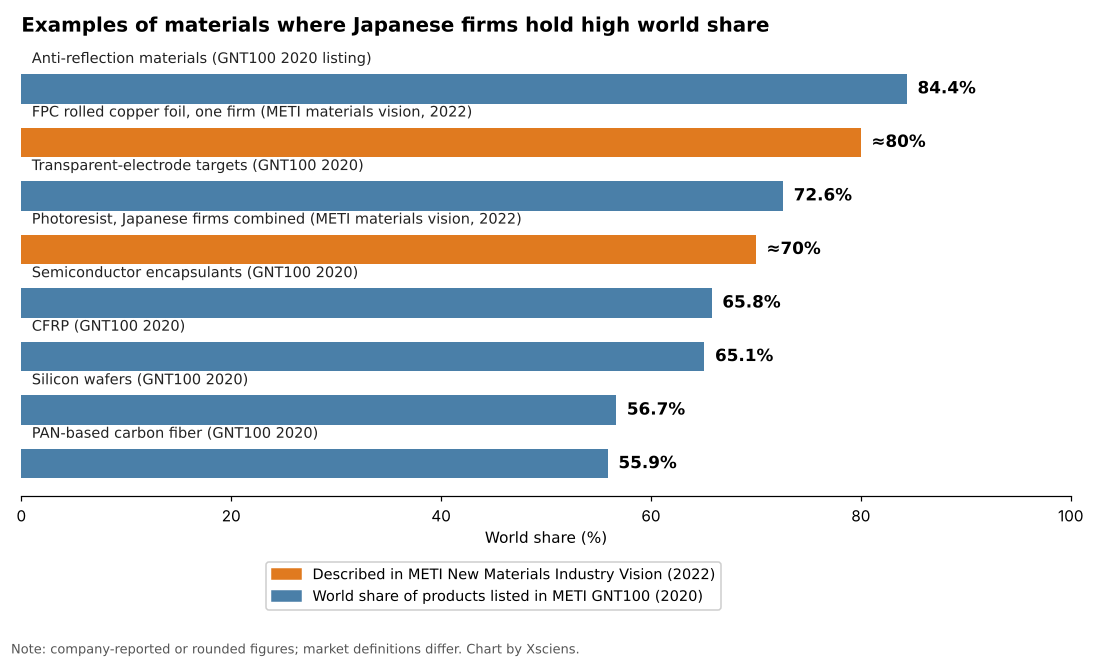
    According to the interim summary of METI’s New Materials Industry Vision (June 2022), materials account for 20% of Japan’s manufacturing GDP and support 220,000 jobs in steel and 940,000 in chemicals. Japanese firms hold 70% of the world market for photoresist, the chemical used to print circuits onto chips, and one company, Company A, holds 80% of rolled copper foil for flexible printed circuits (FPCs), the bendable wiring in smartphones. The Cabinet Office’s Materials Innovation Strategy (June 2025), citing a NEDO survey, also notes many materials with world share above 60%.

    The strength shows in profits as well as share. METI’s 2020 Global Niche Top Companies 100 selected 113 firms from 249 applicants. Their average world share was 43.4% and their average operating margin 12.7%, well above the 4.8% manufacturing average (fiscal 2018). In materials and chemicals alone, the margin was 13.9% and the average share 50.6%.

    Bar chart of materials and components where Japanese firms hold high world shares, ranked by share
    Source: Chart by Xsciens based on METI, New Materials Industry Vision interim summary (2022) and METI GNT100 (2020). Orange bars are figures described in the METI vision; blue bars are products listed in GNT100. Some values are company-reported or rounded and market definitions differ, so bars are not strictly comparable.

    There are challenges too. The same METI document shows China’s share of world crude steel output rising from 15% in 2000 to 53% in 2020. The Cabinet Office’s 2025 strategy lists stagnant paper counts, a declining international presence, a shortage of people who can run data-driven materials development (materials informatics, MI), and slow social implementation. NISTEP reports that, on a fractional-count basis, Japan’s Top10% and Top1% adjusted paper counts in chemistry, materials science and basic life sciences fell by 20% or more between 2010 and 2020. PwC Japan’s analysis points to the small scale of high-share businesses, low overseas sales ratios and a “valley of death” between research and commercialization.

    What industry structure do materials sit in?

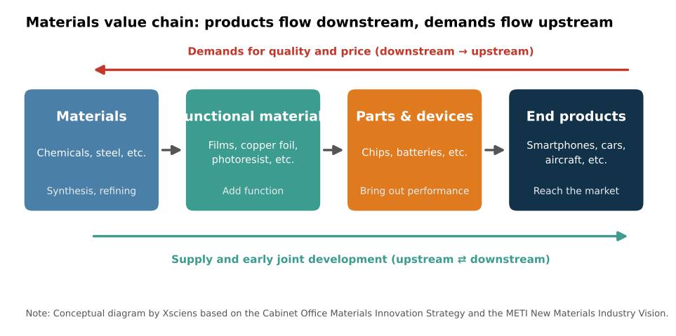
    Materials are inconspicuous in the final product. The Cabinet Office strategy describes materials as both “constituents of end products and the source of their functions.” Material makers produce functional materials such as films, copper foil and photoresist; parts makers use them in chips and batteries; and finally smartphones, cars and aircraft are completed. Along this chain, material makers face demanding quality and price requirements from downstream industries. METI describes meeting them as the foundation of other industries’ competitiveness.

    Diagram of the value chain from materials to functional materials, parts and devices, and end products, with quality and price demands flowing upstream and early joint development linking both ends
    Source: Conceptual diagram by Xsciens based on the Cabinet Office Materials Innovation Strategy and the METI New Materials Industry Vision.

    Sitting there, materials have an impact far beyond their cost. For Ajinomoto’s ABF, an insulating film used in semiconductor packages, a GIGAZINE article of April 2026 reports that it makes up less than 0.1% of the product price, yet its share is close to 100%, and surging demand for AI chips could create shortages. The Cabinet Office strategy likewise says Japan has many items with very high world share that hold an indispensable place in global supply chains.

    Why the hypotheses matter

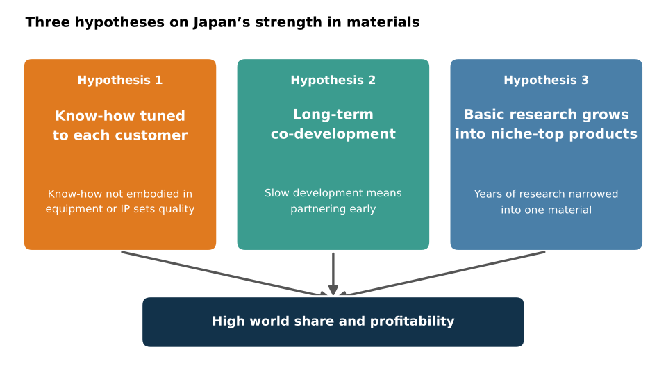
    Strength in materials does not stay in visible form like equipment or patents. Unless we ask why Japan is strong, we cannot see what to protect or what to build on next. The Cabinet Office strategy names “suriawase-type development” (close tuning with the user), the know-how of evaluation, analysis, processing and synthesis, and strong industry-academia ties as Japanese strengths, and stresses long-term investment because materials R&D takes a long time. From this we organize the reasons into three hypotheses.

    Concept diagram: know-how tuned to each customer, long-term co-development, and basic research growing into niche-top products lead to high world share and profitability
    Source: Concept diagram by Xsciens based on the cited documents.

    Hypothesis 1 is shop-floor “suriawase”: polishing a product to each customer. Hypothesis 2 is long-term co-development: partnering early with downstream customers and growing a product over years. Hypothesis 3 is that years of basic research grow into niche-top products focused on one material. Below, we look at why each matters and how it works in practice, using a different company for each.

    Hypothesis 1: shop-floor “suriawase” tuned to each customer

    The best conditions for a material differ with each buyer’s process. METI’s document says that “know-how not embodied in equipment or intellectual property is the source of the materials industry’s strength.” Equipment and patents can be bought or studied, but know-how built up in people and organizations is hard to copy from outside. The Cabinet Office strategy also calls evaluation, analysis, processing and synthesis techniques “a mass of know-how.” That is why hypothesis 1 matters: it is a source of resistance to imitation.

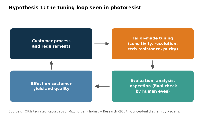
    In practice, take TOK (Tokyo Ohka Kogyo), a photoresist maker. Its 2020 integrated report describes its strength as the ability to quickly deliver tailor-made photoresists, fine-tuned to each customer’s needs and each process’s requirements. The performance factors include sensitivity, resolution, etch resistance and purity, and the report says photoresist greatly affects a customer’s quality and yield. TOK is ranked first in the world for semiconductor photoresist, with a 25.6% share by projected 2020 shipment volume.

    Loop showing customer process and requirements, tailor-made tuning, evaluation, analysis and inspection, and the effect on customer yield and quality
    Source: Conceptual diagram by Xsciens based on TOK Integrated Report 2020 and the Mizuho Bank Industry Research report (2017).

    A 2017 report by Mizuho Bank’s Industry Research Division names two common strengths of Japanese material makers, the ability to develop products to customer needs and efficient, stable production operations, and says they have prized inspection steps where “in the end, people check by eye” to meet demanding domestic customers. Receive the customer’s requirement, tune, inspect, return. Repeating this loop for years builds up as shop-floor know-how.

    Hypothesis 2: long-term co-development with downstream customers

    Materials R&D takes a long time. The Cabinet Office strategy therefore calls for research and development in which upstream and downstream industries cooperate from the early stages. Partnering with customers early and growing uses together makes a material a lasting part of the customer’s product. That is why hypothesis 2 matters.

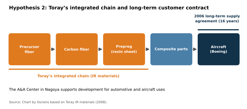
    The practice shows in Toray’s carbon fiber. According to Toray’s investor materials, the company signed a 16-year long-term carbon-fiber composite supply agreement with Boeing in 2006. An ITmedia article (February 2009) reports that this was an exclusive contract under which Boeing buys the 787’s structural carbon fiber from Toray alone, and that Toray kept developing carbon fiber for about 40 years while accepting losses, selling it for golf clubs and the like while pursuing aircraft certification. Its model is integrated production from precursor fiber through carbon fiber to prepreg (resin-impregnated sheet). In Nagoya it set up the A&A Center, a technology development site that includes the AMC for automotive uses (opened June 2008) and the ACC for composite product development (scheduled to open April 2009). In the same document Toray projected a world carbon-fiber share of about 37% after its capacity expansion (a 2008 plan).

    Flow from precursor fiber to carbon fiber, prepreg, composite parts and aircraft (Boeing), with the 2006 long-term supply agreement
    Source: Chart by Xsciens based on Toray IR materials (2008).

    Looking from material to composite to the customer’s airframe, and promising supply under a 16-year contract: the length of this relationship becomes the base for growing uses together with the customer.

    Hypothesis 3: basic research grows into niche-top products

    Materials research takes years to become a product. The Cabinet Office strategy calls Japan’s materials field one with relatively strong industry-academia ties and, on the principle that “industry is the dojo of scholarship,” seeks to advance social implementation and deeper science together. A path that grows accumulated basic research into products focused on one material is why hypothesis 3 matters.

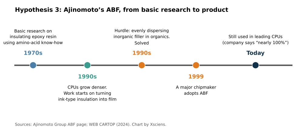
    The practice shows in Ajinomoto’s ABF. According to the Ajinomoto Group, in the 1970s it continued basic research on insulating epoxy resin using its amino-acid know-how. In the 1990s, as CPUs grew denser and pin counts rose from an early 40 to over a thousand, a new insulating material for circuit boards was needed. As a latecomer, Ajinomoto took on the task of turning an ink-type insulating material into a film. The hurdle was mixing organic matter (epoxy resin and hardener) with inorganic filler and dispersing it evenly, which the research team solved to make a thermosetting film. A major chipmaker adopted it in 1999, and it is still used in leading CPUs. The company offers customers the processing method as a system, including optimized laser drilling and copper plating.

    Timeline of Ajinomoto’s ABF from 1970s basic research through 1990s filming, 1999 adoption, and today
    Source: Chart by Xsciens based on the Ajinomoto Group ABF page and WEB CARTOP (2024).

    WEB CARTOP (June 2024) also reports that ABF’s history begins with amino-acid R&D in the 1970s. It is a case where basic research that began in the 1970s met a market need in the 1990s and became a product. The same flow shows in Akira Yoshino, who shared the 2019 Nobel Prize in Chemistry. According to the Nobel Foundation, the prize was shared with Whittingham and Goodenough “for the development of lithium-ion batteries,” and Yoshino’s affiliations were Asahi Kasei and Meijo University. Corporate and university research came together in a battery product.

    Outlook: keeping the edge

    According to METI, materials industries such as steel and chemicals account for about 80% of industrial CO₂ emissions, so in a decarbonizing world, materials that cut emissions are themselves a competitive asset. The way materials are developed is also changing. METI cites a catalyst developed with Yokohama Rubber in which MI achieved a world-best yield (60–70%) and a catalyst matching the performance of crude-oil-derived tires. The Cabinet Office notes that DeepMind predicted about 2.2 million stable compounds. Turn hypothesis 1’s shop-floor know-how into data, extend hypothesis 2’s customer ties to new uses, and sustain hypothesis 3’s basic research. Whether Japan can overlay all three is the key to the next decade. For an example of basic materials chemistry, see our article Ammonia From Air Under Milder Conditions: Kyoto University and Others Explain Why a Molybdenum Catalyst Works.

    Xsciens Editorial Note

    Japan’s strength in materials is easier to understand as accumulated strength in which three hypotheses overlap, rather than a single cause.

    • Read share figures with definitions and dates aligned. For photoresist, Japanese firms combined are 70% in METI’s document, about 90% in PwC Japan’s analysis, and TOK alone is 25.6% (projected 2020 shipments), so figures differ by source. The GNT100 figures include company-reported values. When comparing, check the source, year and market scope.
    • The three hypotheses are not proof of causation. They are leading views drawn from documents and cases, and we found no study that separates how much each one contributes. TOK, Toray and Ajinomoto are all success stories, and the same path may not apply to every material.
    • The base of the strength is past accumulation, with no guarantee for the future. Ajinomoto’s ABF is a case where basic research that began in the 1970s became a product in the 1990s. If highly cited papers are now declining and materials-development talent is short, the effect may show in a few years.
    • From the editors — the smartphone and battery you use every day are made of layers of materials whose names you may never have heard. Knowing that Japanese firms support a number of them may change how you read the next “new material” headline. Still, strength does not last by itself. Take pride in today’s numbers, and keep an eye on whether investment in research and people continues.

    References for this note: PwC Japan analysis of the chemicals industry (scale of high-share businesses, valley of death), Mizuho Bank Industry Research, “Materials” (2017), ITmedia Business Online (February 2009), WEB CARTOP (June 2024), NISTEP RM329 press release (international paper comparison)

    Sources: METI, New Materials Industry Vision interim summary (2022), Cabinet Office, Materials Innovation Strategy (2025), METI GNT100 2020, TOK Integrated Report 2020, Toray IR materials, ITmedia Business Online (February 2009), Ajinomoto Group ABF, GIGAZINE (April 2026), Nobel Foundation (2019 Chemistry), PwC Japan, NISTEP RM329

  • [Science] What Is Backpropagation? A Simple Guide to How AI Learns

    [Science] What Is Backpropagation? A Simple Guide to How AI Learns

    Backpropagation is the algorithm that lets artificial neural networks learn from their own mistakes, and it quietly powers much of today’s AI — from chatbots that answer your questions to the apps that recognize a face in a photo. Understanding it, even at a basic level, is one of the clearest ways to understand how modern deep-learning systems actually learn.

    Original Paper

    Title: Learning representations by back-propagating errors
    Authors: David E. Rumelhart, Geoffrey E. Hinton, Ronald J. Williams
    Journal: Nature, Vol. 323, pp. 533–536 (1986)
    DOI: 10.1038/323533a0

    What Is Backpropagation, Exactly?

    In plain terms, backpropagation — short for “backward propagation of errors,” also known as error backpropagation — is a method for training a neural network by repeatedly working out how wrong its answer was, and in which direction each connection should adjust. A neural network is built from layers of simple, interconnected units (loosely inspired by neurons) joined by adjustable connection strengths called weights. When a network is first created, its weights are usually set to small, carefully chosen random values, so its first guesses are generally poor. Backpropagation is the procedure that turns that rough starting point into a network that can recognize a cat in a photo, translate a sentence, or predict the next word in a reply.

    There is one important distinction worth keeping straight: backpropagation calculates how much each connection contributed to the error, while a separate step called gradient descent uses that information to actually adjust the connections. People often use “backpropagation” loosely to describe the whole training process, but technically the two are different steps working together.

    How the Algorithm Actually Works

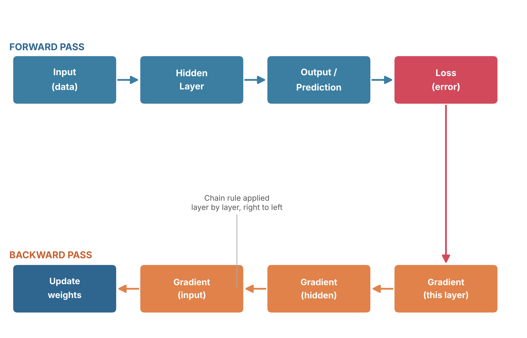
    Training with backpropagation happens in two passes. In the forward pass, an input — a photo, a sentence, a row of sensor data — moves through the network’s layers in order, and the network produces a prediction. That prediction is then compared with the correct answer using a loss function, a numerical measure of how far the prediction was from the desired result.

    Backpropagation doesn’t tell a network what to think. It tells the network how wrong it was, and in which direction each connection should move to be a little less wrong next time.

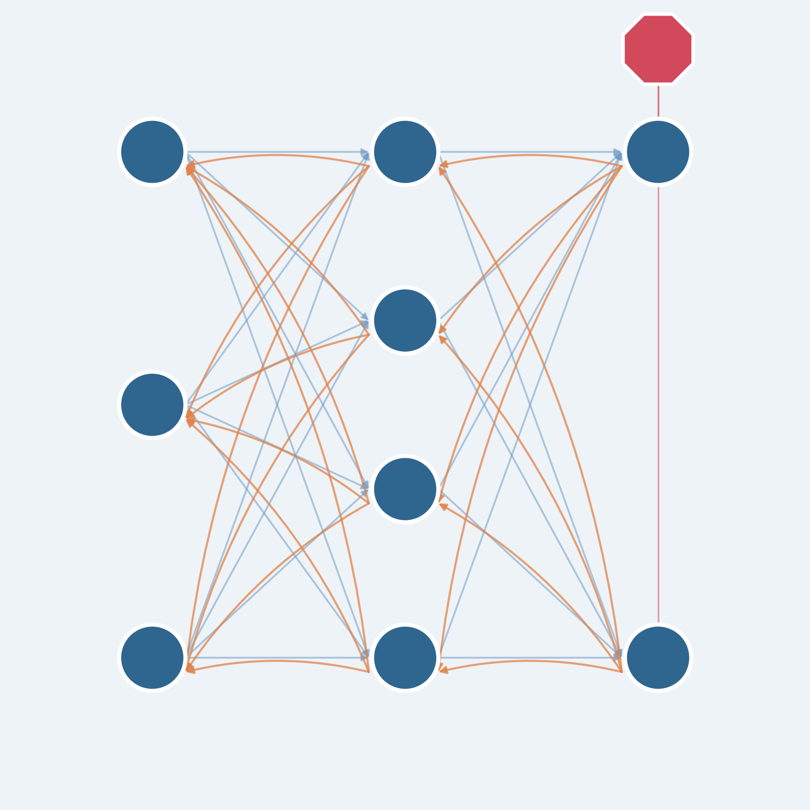
    A simple analogy helps before the math: imagine a product moving through several stages of a factory line, and the finished item turns out defective. To find the cause, managers work backward from the end of the line, and each stage reports how much it may have contributed to the problem, passing that information to the stage before it. The backward pass in backpropagation does something similar, except it uses calculus to work this out exactly. Starting at the output layer and moving back toward the input, the algorithm applies the chain rule — a technique for tracking how a change at one stage ripples through a chain of dependent calculations. Each layer combines information about how its own calculations affected the next layer with the error information passed back from that layer, producing a gradient: a measure of how sensitive the loss is to a small change in each weight, at its current value.

    Diagram of the forward pass and backward pass in backpropagation
    The forward pass produces a prediction and a loss; the backward pass applies the chain rule, layer by layer, to compute gradients and update the weights.

    Once every weight has a gradient, gradient descent uses it to actually update the weights, nudging each one a small amount in the direction that reduces the error. Repeat this forward-pass/backward-pass/update cycle over thousands or millions of examples, and a network that started with randomly initialized connections gradually comes to reflect real structure in the data. The appeal of backpropagation is efficiency: it calculates gradients for every weight in a network in roughly the time needed for a small number of forward and backward passes, rather than requiring a separate experiment for each individual weight.

    Why Backpropagation Is Getting Attention Again

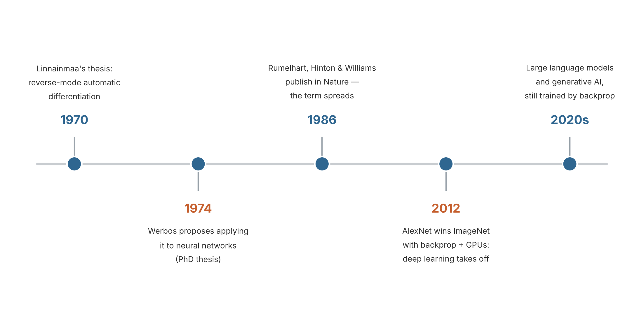
    Backpropagation is not new, and its mathematical core had already been explored before it became famous. Reverse-mode automatic differentiation — the calculus technique at the heart of the algorithm — traces back to Finnish researcher Seppo Linnainmaa’s 1970 master’s thesis, and American researcher Paul Werbos proposed applying a related idea to neural networks in his 1974 doctoral thesis. The method became particularly influential after David Rumelhart, Geoffrey Hinton and Ronald Williams published “Learning representations by back-propagating errors” in Nature in 1986, demonstrating that it could let multilayer networks automatically discover useful internal features rather than relying entirely on engineers to design them by hand.

    For years afterward, backpropagation-trained networks were mostly a research curiosity, limited by available data and computing power. That changed dramatically in 2012, when Alex Krizhevsky and Ilya Sutskever, working with their advisor Geoffrey Hinton, combined backpropagation, the large labeled ImageNet dataset, and graphics-card computing power in a network known as AlexNet. It dramatically outperformed competing approaches in that year’s ImageNet image-recognition competition, a result widely credited with triggering the modern deep learning boom. The large language models behind today’s generative AI chatbots are, at their core, still trained with variations of the same algorithm.

    Timeline of key milestones in the history of backpropagation, from 1970 to the 2020s
    Source: created based on Linnainmaa (1970), Werbos (1974), Rumelhart, Hinton & Williams, Nature (1986), and the AlexNet/ImageNet milestone (2012).

    What has put backpropagation back in the spotlight recently is a different question: does the brain do anything like this? In October 2026, a team at MIT’s McGovern Institute, led by Qianli Liao, Liu Ziyin and Yulu Gan with senior authors Mark Harnett and Tomaso Poggio, published a study in the Proceedings of the National Academy of Sciences proposing a computational model in which randomly connected artificial networks can self-organize their own forward and feedback pathways, using only local learning rules inspired by biological synapses and no global error signal — and still learn nearly as well as backpropagation on the tasks tested. The researchers are careful to frame this as a candidate mechanism and a testable hypothesis, not proof that real brains work this way, but it reopens a question that has nagged neuroscientists for roughly 40 years: backpropagation is clearly powerful enough to drive today’s AI, yet nothing in a biological brain has been shown to do precisely what it requires. (Related article: A Simulated Brain Circuit Builds Its Own AI-Like Learning System, MIT Finds.)

    Where You’ve Already Met Backpropagation

    Even though the math stays behind the scenes, the results of backpropagation-trained networks are part of ordinary life. Many modern face-unlock features and the photo apps that automatically group pictures of the same person run on neural networks trained with backpropagation or related gradient-based methods. Voice assistants that transcribe speech or answer spoken questions generally rely on networks trained the same way. Generative AI chatbots are also built using neural networks trained with backpropagation — during an early stage called pretraining, for example, a language model repeatedly tries to predict the next word in a passage of text, compares its guess with the actual word, and adjusts its weights to reduce the error; later training stages then refine how it follows instructions and responds to feedback.

    It’s worth keeping one distinction in mind: backpropagation mainly happens during training, not every time you use these tools. Once a network has learned, it typically uses its already-adjusted weights to make predictions, without recalculating gradients or updating itself each time — the heavy lifting happened earlier, often across billions of training examples.

    What to Watch Next

    Backpropagation itself is a mature, well-understood technique, so the open questions now sit in its limitations and the alternatives researchers are exploring. One is scientific: whether the MIT team’s self-organizing, locally-plausible learning circuits — or related approaches sometimes called feedback alignment or predictive coding — can be tested directly against real neural tissue, and whether they can match backpropagation’s performance on problems much larger than the ones tested so far. Another is practical: as AI models keep growing, researchers continue to look for training methods that need less computing power than standard backpropagation while keeping its accuracy. The next breakthrough may not come from making backpropagation itself faster, but from discovering how networks can learn without depending on it so completely — which is exactly the question AI researchers and neuroscientists are now asking together.

    Xsciens Editorial Note

    Backpropagation is best understood as a precise bookkeeping trick for calculating how a network should adjust itself, not as a theory of how any brain, artificial or biological, actually “thinks.”

    • A common misconception. “Neural network” learning is often described as though it copies how the brain learns, since artificial “neurons” were loosely inspired by biological ones. In practice, standard backpropagation’s backward calculation relies on precise weight-related information tied to the exact connections used for forward signaling — something no real neuron is known to reproduce or transmit in the same way. (Some alternative methods, such as feedback alignment, relax this requirement, which is itself a sign of how specific the original objection is.) The resemblance between artificial and biological “neurons” is a loose analogy, not a working description of what either one computes.
    • Limits and open questions. A common misreading is that backpropagation always needs a human-provided “correct answer,” like a teacher grading homework. That’s not quite right: it needs a differentiable training objective, which can come from supervised labels, but also from self-supervised tasks (such as predicting the next word in a sentence) or reinforcement-style rewards. What backpropagation does not explain, on its own, is why some network architectures generalize well to new data and others don’t, or how an AI system might decide what is worth learning in the first place — those remain active, only partly answered research questions, not settled ones.
    • What to watch next. The MIT team’s October 2026 study proposes, as a specific and testable hypothesis, that a four-synapse wiring motif linking ascending and descending pathways in the cortex could let real circuits self-organize a similar learning ability. This is a model prediction, not a confirmed feature of brain tissue — whether neuroscientists actually find that wiring pattern, and whether locally-plausible learning rules can match backpropagation’s performance on problems far larger than the ones tested so far, are the two developments worth watching.
    • From the editors — If brain-inspired, locally-learning AI matures the way this MIT team hopes, the assistants people use every day could stop feeling like blank tools that need re-explaining each time and start quietly adapting to how each person actually works. Getting there would likely mean systems that keep adjusting themselves after they leave the lab, learning from ordinary daily use instead of one big retraining cycle. That same ability to keep learning on its own is exactly what to watch: without a way to check what a system has quietly picked up, it could just as easily drift toward learning the wrong lesson from unusual or misleading experience. This is still an early computational demonstration, not a finished product — so if an assistant ever starts to feel like it “gets” you a little faster, it’s worth asking, every so often, what it actually learned to get there.

    References for this note: Quanta Magazine — Artificial Neural Nets Finally Yield Clues to How Brains Learn, arXiv — Brain-Inspired Machine Intelligence: A Survey of Neurobiologically-Plausible Credit Assignment

    Sources: IBM — What Is Backpropagation?, TechTarget — What Is a Backpropagation Algorithm?, Rumelhart, Hinton & Williams, Nature (1986), Seppo Linnainmaa, Computer History Museum — AlexNet Source Code, Xsciens — A Simulated Brain Circuit Builds Its Own AI-Like Learning System, MIT Finds

  • [Science] Hidden Crystal “Patchwork” Could Help Explain Why Superconductors Differ

    [Science] Hidden Crystal “Patchwork” Could Help Explain Why Superconductors Differ

    A copper-oxide superconductor that scientists have studied for about 40 years turns out not to be uniform inside. A University of Warwick team used 3D X-ray imaging to show that one well-known crystal is a patchwork of two slightly different atomic arrangements, divided by boundaries roughly 150 nanometres wide. That matters because most theories of these materials quietly assume a uniform crystal, and the hidden boundaries might help explain why seemingly identical samples can perform differently.

    原論文情報 / Original Paper
    Title: Giant Domain Walls and Intrinsic Heterogeneity in 214 Cuprate Superconductors
    Authors: Ladbrook, E., Wright, J. P., Senn, M. S.
    Journal: Physical Review Letters 137(12), 2026
    DOI: 10.1103/r62x-kt5j

    What the team found

    Copper-oxide superconductors, or cuprates, were discovered in 1986. They carry electricity with zero resistance at temperatures far higher than older superconductors, although still very cold by everyday standards. Four decades on, their behaviour remains only partly understood. Researchers have long known that cuprates can be uneven in their electronic behaviour, but many interpretations have still treated the underlying crystal structure as essentially the same all the way through. How different structural regions are arranged throughout the bulk of a crystal has remained unclear.

    The new study, led by Mark Senn at the University of Warwick with Evie Ladbrook and Jon Wright of the European Synchrotron Radiation Facility (ESRF) in France, tested that assumption directly. The sample was a tiny single crystal with the composition La₁.₆₇₅Eu₀.₂Sr₀.₁₂₅CuO₄. It belongs to the “214” family of copper-oxide compounds and is doped to one-eighth, meaning roughly one added charge carrier for every eight copper atoms in its copper-oxide layers, a level at which superconductivity is known to be fragile. Inside it, the researchers found regions with two closely related atomic arrangements, separated by walls far broader than expected.

    How you photograph the inside of a crystal

    The tool was scanning 3D X-ray diffraction, which works a little like a CT scan. At ESRF’s ID11 beamline, the team focused an X-ray beam to about 120 nanometres and scanned it across the crystal in 50-nanometre steps. The crystal was also rotated so that diffraction data came from many angles, and each scan took about two hours. From the positions of the diffraction spots, the team reconstructed how the crystal lattice is stretched or twisted from place to place, with a strain sensitivity of roughly two parts in ten thousand. Beyond superconductors, the same approach could be used to look for hidden structural variations in other complex materials.

    The Warwick press release credits a recent €150 million upgrade of the ESRF for making this kind of measurement practical. In the paper’s own words, the technique offers a general way to resolve the bulk microstructure of materials, not just superconductors.

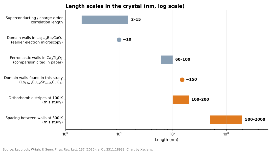
    Bar chart on a log scale comparing the 150 nm domain walls found in this study with other length scales in cuprates
    Source: Ladbrook, Wright and Senn (2026), Physical Review Letters; arXiv:2511.18938. Chart by Xsciens.

    Walls broader than anyone expected

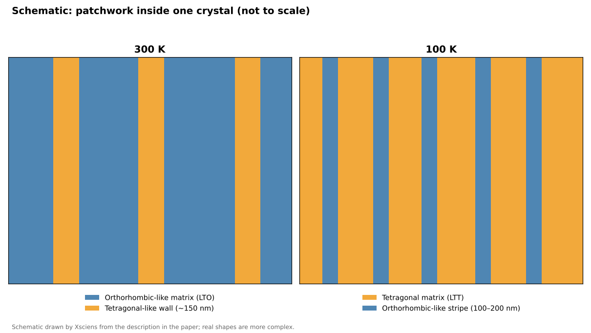
    At room temperature (300 K) the crystal is mostly in a so-called orthorhombic state, in which the lattice is slightly stretched along one in-plane direction, with two orientations of twin domains (regions of the same structure rotated relative to each other) each a micron or more across. Between them the team saw wall regions about 150 nanometres thick, spaced roughly 0.5 to 2 micrometres apart, where the measured orthorhombic strain approaches zero. In other words, the walls look more like a different, tetragonal-like structure, one with equal lengths along both in-plane directions, than like thin seams between two orthorhombic domains.

    For comparison, earlier electron-microscopy work on a related compound, La₂₋ₓBaₓCuO₄, estimated the width of similar regions at only around 10 nanometres, and the correlation lengths of superconducting and charge-density-wave order in cuprates are typically about 2 to 15 nanometres. (Charge order is a pattern in which electrons gather in regularly repeating regions instead of spreading evenly.) The comparison is rough, since the compounds and techniques differ, but it suggests the new walls are not tiny imperfections: they are broad enough to behave almost like a structure in their own right. Professor Senn said that for forty years the working assumption had been that these materials are the same all the way through.

    Cooling reshapes the pattern

    The picture changes as the crystal is cooled. This material is known to switch around 160 K from the orthorhombic state to a low-temperature tetragonal one, and the team measured it at 300, 140, 120 and 100 K. At 100 K they saw the reverse arrangement: fine stripes of orthorhombic-like material, each roughly 100 to 200 nanometres wide, embedded in a tetragonal matrix. So the pattern does not simply become more uniform on cooling; the dominant structure changes while smaller regions of the other one remain embedded in it. Earlier studies have reported that this kind of coexistence persists down to at least 10 K in this material and a related barium compound, but the new X-ray measurements went no lower than 100 K.

    Schematic showing tetragonal-like walls in an orthorhombic matrix at 300 K and orthorhombic-like stripes in a tetragonal matrix at 100 K
    Schematic by Xsciens based on the description in the paper; not to scale.

    Why it matters, and what is not yet shown

    The idea that structure and superconductivity interact in this family is not new. In 1995, a neutron-scattering study on a related compound near one-eighth doping linked a static pattern of alternating spin and charge stripes to the suppression of superconductivity there. What the Warwick work adds is a three-dimensional, micrometre-scale view of how the crystal structure itself is divided up, and the finding that the dividing walls are much wider than the sharp seams people tended to picture.

    The authors suggest the tetragonal-like boundaries could influence the competition between superconductivity and charge order, and Professor Senn says they probably work against superconductivity rather than alongside it. If so, that could help explain why some cuprates outperform others and why bulk measurements sometimes disagree. Understanding why some cuprates superconduct better than others has been a longstanding challenge, so the way structural regions are arranged may be one more factor to consider alongside chemical composition. The authors also expect similar patchwork in the wider 214 family, and possibly in related materials studied under extreme pressure. If so, some past bulk measurements may need reinterpreting.

    Those are hypotheses, not results. The experiment measured crystal structure, not electrical behaviour: superconductivity at the walls was not measured directly, and the paper describes the link as suggestive. Only one micro-crystal was measured, the apparent wall width depends on the instrument’s resolution, and the faint charge-order signals cannot yet be mapped with this method.

    Xsciens Editorial Note

    One carefully imaged crystal shows that the “same all the way through” assumption fails in at least one well-studied cuprate.

    • What was observed versus what was inferred. The observation is a three-dimensional map of structural distortion: tetragonal-like walls about 150 nm thick at 300 K and orthorhombic-like stripes in a tetragonal matrix at 100 K. That the walls suppress superconductivity is an interpretation, not a direct measurement, and the paper calls the evidence suggestive.
    • The sample is tiny and single. The result comes from one crystal about 15 × 20 × 20 micrometres of one composition. The authors state that extending it to other cuprates is a prediction, and measured wall widths depend on the instrument’s resolution (roughly 30–70 nm).
    • What to watch next. The key test is whether superconductivity is weaker inside the walls themselves or whether the walls affect the surrounding crystal. That needs structural imaging combined with local electrical measurements, including charge order, repeated on other cuprates.
    • From the editors — superconductors that are easier to make and work better could one day mean leaner power grids and smaller, cheaper MRI scanners in more hospitals. The route there may run through treating the arrangement of a crystal’s internal regions as a design dial, alongside its chemical recipe, although removing every wall might not even help. But a tidy lab crystal is a long way from an affordable wire. So when a superconductor headline promises a revolution, ask how large the sample was and what was actually measured.

    References for this note: Keimer et al., “From quantum matter to high-temperature superconductivity in copper oxides,” Nature (2015), Tranquada et al., “Evidence for stripe correlations of spins and holes in copper oxide superconductors,” Nature (1995)

    Sources: University of Warwick press release, Physical Review Letters (DOI 10.1103/r62x-kt5j), arXiv:2511.18938

  • [Science] The Brain’s Alertness System Has More Specific Wiring Than Scientists Thought

    [Science] The Brain’s Alertness System Has More Specific Wiring Than Scientists Thought

    Norepinephrine, a brain chemical involved in alertness, attention and stress responses, comes largely from a tiny cluster of cells in the brainstem called the locus coeruleus (LC). For decades this system was often pictured as a foghorn, broadcasting much the same signal everywhere. A new Nature study in mice, led by researchers at the Allen Institute, finds a more organized picture, closer to a postal network: different LC neurons tend to send norepinephrine to different destinations and show different activity during behavior. Why it matters: some medications for depression and ADHD influence norepinephrine signaling, and a wiring map is a first step toward understanding how the system could one day be influenced more selectively.

    原論文情報 / Original Paper
    Title: Topographic structure and function of locus coeruleus noradrenaline neurons
    Authors: Zhixiao Su, Polina Kosillo, Kanghoon Jung et al.
    Journal: Nature (2026)
    DOI: 10.1038/s41586-026-11026-0

    What the locus coeruleus does

    The locus coeruleus (LC) is a tiny brainstem nucleus, often nicknamed the “blue spot,” and the main source of norepinephrine, also called noradrenaline, for much of the brain and spinal cord. The chemical helps regulate arousal, attention and mood, and some medications for depression and ADHD act on norepinephrine signaling. Changes in the LC have also been reported early in Alzheimer’s disease, although the timing and significance of that degeneration are still under study.

    The textbook picture often treated the LC as a broadly broadcasting system, rather like a foghorn. Earlier work had already hinted at more structure. A 2020 review in Nature Reviews Neuroscience, for example, concluded that subgroups of LC neurons can encode specific cognitive processes, and a 2023 eLife study found two main electrical and structural cell types in the mouse LC. The new study maps how those differences in wiring, gene expression and activity are organized across the structure.

    Mapping one tiny structure

    Why map a structure this small? Because a nucleus that reaches almost the entire brain is hard to understand from the outside. Unless researchers know which neurons talk to which regions, it is difficult to say whether a drug, a stress response or a behavior is engaging the whole system or only a piece of it. Anatomy comes first, and function can be tested against it.

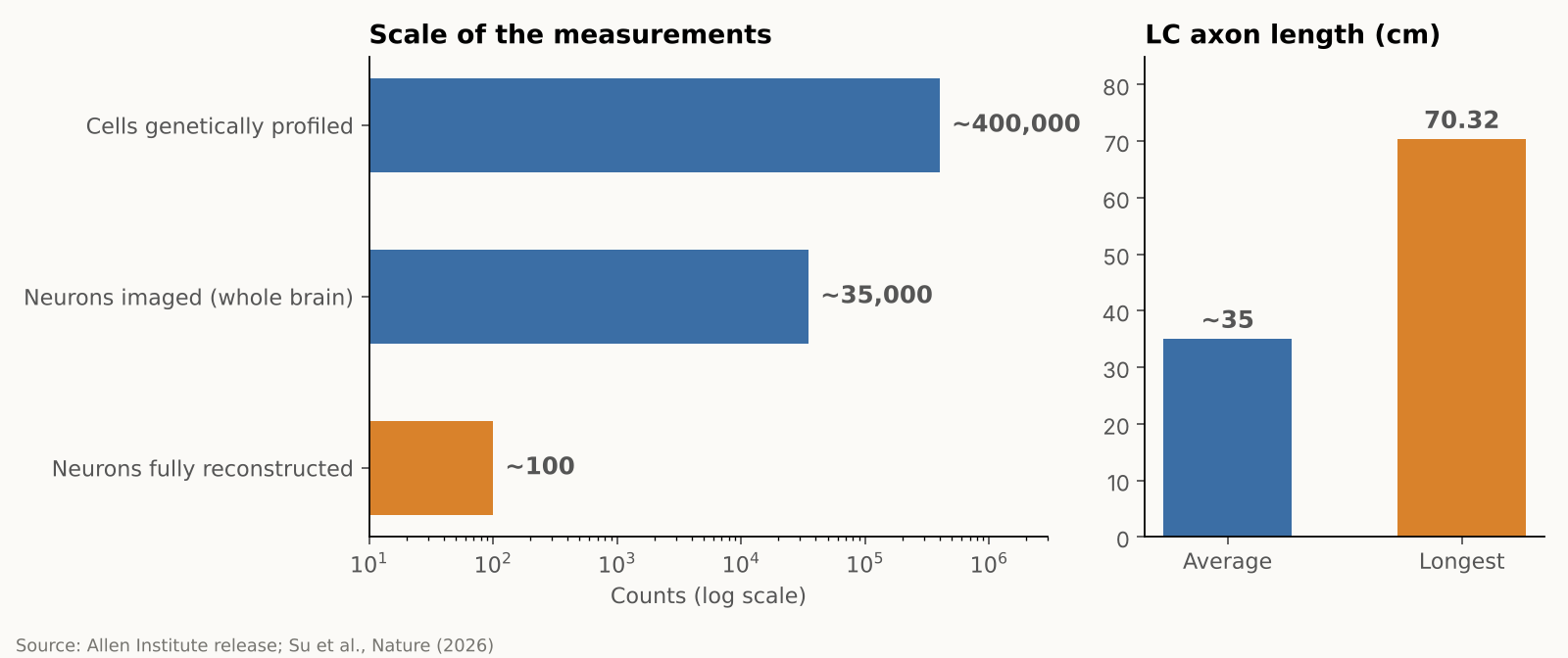
    The team combined several approaches in mice, each answering a different question. Whole-brain imaging showed where LC neurons send their fibers, gene profiling showed which genes they use, and detailed reconstructions traced the branches of individual cells. The researchers then recorded neural activity while mice performed a learning task. In numbers, they imaged almost 35,000 neurons across the whole brain, profiled gene activity in nearly 400,000 cells, and fully reconstructed about 100 individual LC neurons, according to the Allen Institute. These are different measurements from different samples, not 400,000 neurons traced end to end. The research was supported by the NIH BRAIN Initiative.

    Bar charts showing the scale of the measurements and the average and longest LC axon lengths
    Source: Allen Institute news release and Su et al., Nature (2026). Numbers are approximate as reported.

    A map of connections, a gradient of genes

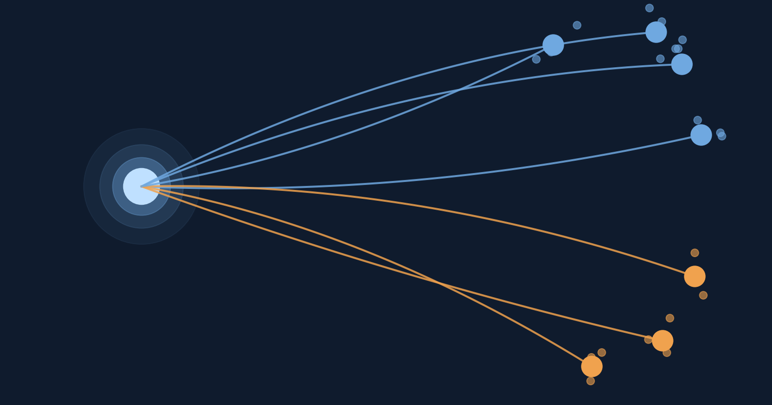
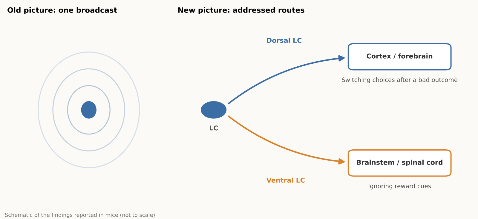
    The reconstructions showed that the LC is organized by position, as a gradient rather than two sealed compartments. Neurons in the upper (dorsal) part mainly send their axons to the cerebral cortex and forebrain, while neurons in the lower (ventral) part mainly project to the brainstem and spinal cord. Gene expression also changes smoothly along that same dorsal-to-ventral axis, matching the projection pattern, according to a summary of the paper’s abstract.

    The striking part is that these patterns line up. A neuron’s position in the LC helps predict where its axon projects and how its gene expression differs from its neighbors, and, in some cases, how it behaves during learning.

    A very long cell, and a selective one

    LC axons, the long fibers that carry signals out of the cell, averaged about 35 centimeters in total length in the mice. The longest one traced measured 70.32 centimeters in total, which the Allen Institute describes as the longest single neuron measured in a mouse. That neuron supplies norepinephrine to a large volume of cortex but does not release it in the cerebellum, brainstem or spinal cord.

    “The findings suggest the brain’s norepinephrine system is far more like a targeted postal network than a foghorn,” said Karel Svoboda of the Allen Institute.

    For readers who follow how the brain learns, this fits a broader theme: learning is not one switch but many coordinated signals. We covered one such idea in our earlier piece on an MIT hypothesis about how the brain might build its own learning circuits.

    Schematic contrasting a single broadcast with two addressed LC routes to cortex and spinal cord
    Schematic based on findings reported in mice. Not to scale.

    Different routes, different jobs

    The activity recordings pointed to different roles. Cortex-projecting dorsal neurons became more active during learning, specifically when mice changed their choice after an unfavorable outcome, and their activity also tracked reward prediction error, the gap between the reward an animal expected and what it actually got, which can guide future choices. Ventral neurons had higher background activity when mice ignored cues indicating that a reward might be available. The authors suggest this may reflect differences in how animals respond to potentially relevant cues.

    A signal that carries that gap is a natural teaching tool. Finding one in a norepinephrine pathway, rather than only in the better-known dopamine system, is why the authors are interested in how the two might work together. They suspect norepinephrine and dopamine may supply complementary learning signals, but that remains a hypothesis. According to The Transmitter, the team plans to study how these chemicals interact next.

    Researchers who were not involved in the work have commented on an earlier preprint version of the study. Nelson Totah of the University of Helsinki called it “bread-and-butter” research for the field that answers basic questions about an evolutionarily ancient structure. Rebecca Jordan of the University of Edinburgh said it suggests the LC could send tailored information to different brain areas, and Robert Froemke of NYU noted that the gene-expression profiling could help researchers record and manipulate specific cell types, according to The Transmitter. The published Nature paper was not evaluated by these experts in that coverage.

    An independent 2025 review adds some context. It summarizes rodent studies in which ventral LC neurons reduced pain through projections to the spinal cord, while activating the LC–prefrontal circuit increased pain and anxiety-like behavior. These results come from separate experiments, but they support the idea that LC pathways can have different effects depending on their destinations.

    Why it matters, and what to keep in mind

    Because norepinephrine-related drugs usually act across the whole brain, a map of separate pathways raises the possibility of more selective ways to influence them that avoid unrelated circuits. The Allen Institute describes this as a possibility for the future, not a demonstrated result. All of the work was done in mice, and nobody has yet shown that human LC neurons are organized the same way. Neither does the study show that any of these pathways can be treated on its own. For now, it is a map, and a good one, rather than a medical advance.

    The practical takeaway for a general reader is modest but real: the brain’s alertness and attention system is more finely organized than the old “one signal for everyone” picture suggested. That kind of basic knowledge tends to pay off slowly, by giving later researchers better targets and better questions.

    Xsciens Editorial Note

    The study suggests that a brain system once treated as a single volume knob is better understood as a network with different destinations. If that view is confirmed in people, treatment for focus and mood, learning support and early detection of brain aging could shift from adjusting the whole brain to targeting only the wires that matter, which may shape the precision of future drugs and diagnostics.

    • What is solid is the map; what is still a hypothesis is the job of each route. Where the axons go, how gene use shifts along the structure, and the recorded activity are direct measurements, so any past interpretation that assumed one broadcast signal now needs revisiting. Reading the dorsal neurons as a “learning signal,” or the ventral ones as tied to responses to reward cues, is an interpretation drawn from how activity lines up with behavior, and the norepinephrine–dopamine partnership remains a hypothesis. These are the claims coming experiments will test.
    • A mouse map is a blueprint; confirming it in people is the next stage. About 100 neurons were reconstructed in full, according to the Allen Institute, and the 35,000 imaged and 400,000 profiled cells are separate measurements. An independent 2025 review also notes that much of the evidence comes from rodents. The flip side is useful: the map tells researchers exactly what to look for in human tissue, which is where the field has to go.
    • Three kinds of study to expect next (our projections). (a) Causal experiments that silence or activate one pathway at a time and see whether behavior changes, a question the study leaves open. (b) Simultaneous recordings of norepinephrine and dopamine to test whether they divide the work of learning, which The Transmitter reports the team plans to study. (c) Studies in human brains, such as post-mortem tissue or imaging, that look for the same dorsal–ventral arrangement.
    • From the editors — the idea of raising or lowering a brain chemical across the board may give way to tuning one wire at a time. This map points to three futures.
      1) Drug design. Today’s norepinephrine-related drugs move the pathway that serves focus and the pathway that drives bodily arousal together. The finding that gene use shifts gradually from dorsal to ventral gives researchers a possible marker for telling routes apart, and an outside expert quoted by The Transmitter noted that gene profiling could help record and manipulate specific cell types. A treatment that nudges the focus-related part without the racing heart and tension is a design goal this map makes more realistic.
      2) Understanding learning. Dorsal neurons responded when mice switched choices and when outcomes missed expectations, which suggests this system may help teach us at the moment we recover from a mistake. If so, the best timing of feedback could become a design question for teaching and rehabilitation. For AI research, the idea of separating a “learn the value” signal from a “change your approach” signal into different wires may be worth borrowing.
      3) Spotting change early. Changes in the LC have been reported early in Alzheimer’s disease. With this map as a ruler, researchers could ask which pathways are damaged first and whether those changes can be caught earlier and in finer detail. This study did not test that.
      These are our projections, and the road from a mouse map to people is still ahead. One way to read the news in the meantime: when you see a headline about a drug that targets a particular brain pathway, check which pathway was tested in humans. That is where a map turns into a treatment, or does not.

    References for this note: McKinney et al., eLife (2023), Hao et al., Int. J. Mol. Sci. (2025), The Transmitter (2026), Poe et al., Nature Reviews Neuroscience (2020)

    Sources: Allen Institute, Su et al., Nature (2026), ScienceDaily

  • [Science] High-Dose Fish-Oil DHA Shifted a Brain Marker but Not Memory, Trial Finds

    [Science] High-Dose Fish-Oil DHA Shifted a Brain Marker but Not Memory, Trial Finds

    A two-year randomized trial found that high-dose DHA, the main omega-3 in fish oil, raised a marker of DHA in the fluid surrounding the brain, yet it did not improve memory-and-thinking scores or slow shrinkage of the memory-related hippocampus compared with placebo. For the many older adults who take fish oil hoping to ward off dementia, the result is a reminder that moving a nutrient into the nervous system is not the same as protecting memory.

    原論文情報 / Original Paper
    Title: CNS target engagement of high-dose DHA supplementation in older adults at risk for dementia: a randomised, double-blind, placebo-controlled trial
    Authors: Yassine HN et al.
    Journal: eBioMedicine 2026;129:106316
    DOI: 10.1016/j.ebiom.2026.106316

    What the researchers tested

    The phase IIa trial, run at the University of Southern California (USC) between September 2018 and May 2024, enrolled 365 adults aged 55 to 80 who did not have dementia, ate little DHA (under 200 mg a day), and had at least one dementia risk factor. About 47% carried APOE ε4, a gene variant that is the strongest common genetic risk factor for late-onset Alzheimer’s disease, although carrying it does not mean a person will inevitably develop the disease.

    Participants were randomly assigned to take either 2 grams of DHA a day or a placebo for 24 months, and neither they nor the staff knew who got which. The work was funded by the U.S. National Institute on Aging and the Alzheimer’s Drug Discovery Foundation, and was published online in June 2026.

    Step one: the marker moved

    The trial’s primary question was whether high-dose DHA could measurably change a biochemical marker of DHA availability in the central nervous system. To check, a subgroup of participants agreed to a lumbar puncture so researchers could sample cerebrospinal fluid (CSF), the liquid that surrounds the brain and spinal cord.

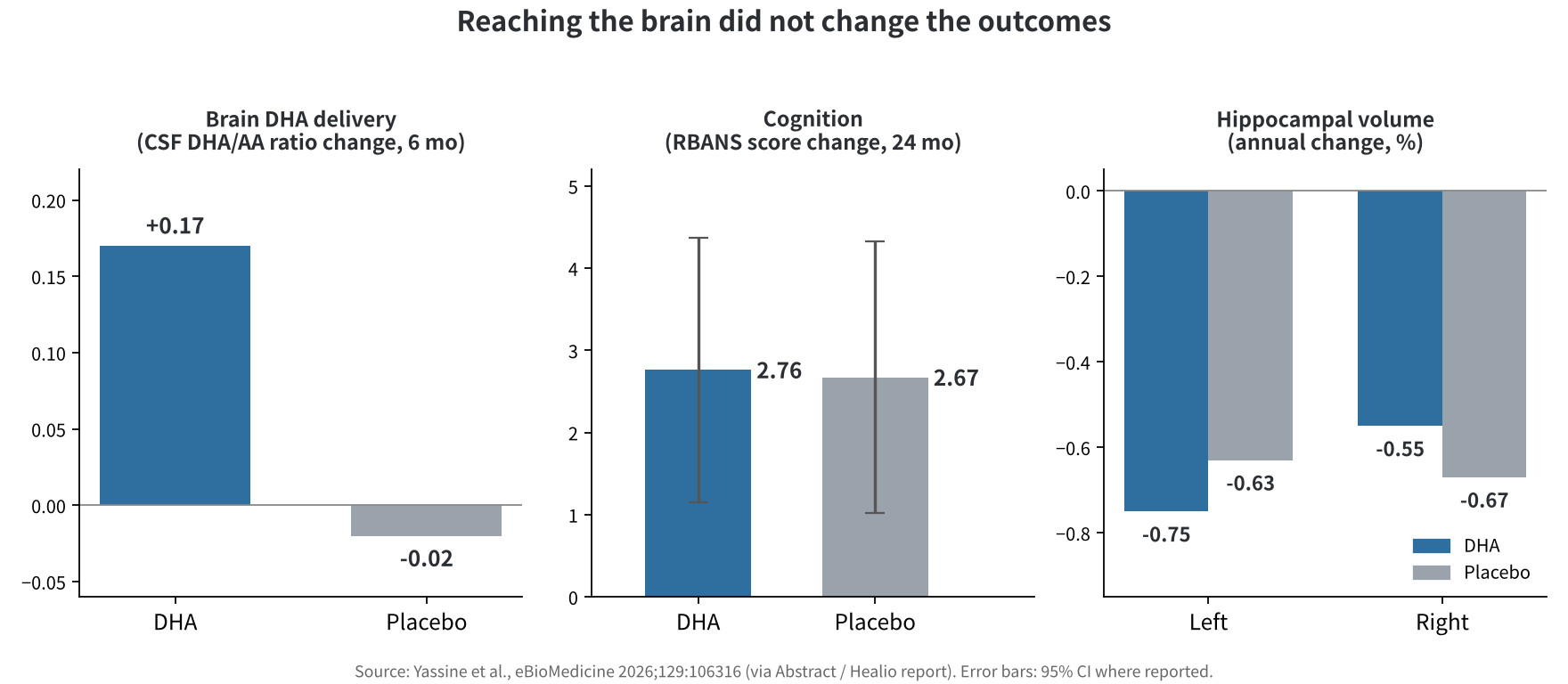
    At six months, the ratio of DHA to arachidonic acid (AA, an omega-6 fat) in CSF had risen by 0.17 in the DHA group and fallen by 0.02 in the placebo group, a difference of 0.19 (95% confidence interval 0.16 to 0.21). The supplement also raised the omega-3 index, a measure of omega-3 fats in red blood cells, from 4.9% to 11%. The CSF increase did not depend on whether participants carried APOE ε4.

    Step two: the outcomes did not

    Cognition and brain structure were secondary outcomes. On a standard memory-and-thinking battery (RBANS), scores rose by 2.76 points in the DHA group and 2.67 in the placebo group. The hippocampus shrank by an estimated 0.75% a year (left) and 0.55% (right) with DHA versus 0.63% and 0.67% with placebo. The authors reported no significant difference between groups for either measure, and side effects were similar, with no serious ones attributed to the supplement.

    Bar charts comparing DHA and placebo: CSF DHA/AA ratio change, RBANS score change and hippocampal volume change
    Figure 1. The brain-fluid marker rose with DHA, but cognition and hippocampal volume looked alike in both groups. Source: Yassine et al., eBioMedicine 2026, and Healio.

    In other words, despite a clear biochemical response, the DHA group did not outperform placebo on the cognitive or structural measures over the two years.

    How to read “no benefit”

    Several caveats matter. About 38% of participants dropped out, mainly because of COVID-19 disruptions. That reduced statistical power and may have introduced bias, because those who left differed from those who stayed, so small effects cannot be ruled out. Participants were also relatively young, well educated and cognitively healthy, so 24 months may be too short to see much decline in anyone. Only one form and dose of omega-3 was tested, and a single supplement may be too little against a disease with many contributing causes.

    The authors argue that future research should prioritize understanding how the brain processes DHA and which people might respond differently. Lead investigator Hussein Yassine said staying active, sleeping well and eating a balanced diet remain the most powerful tools for lowering Alzheimer’s risk. The result also does not say that eating fish is pointless: the study tested a high-dose supplement, not diet.

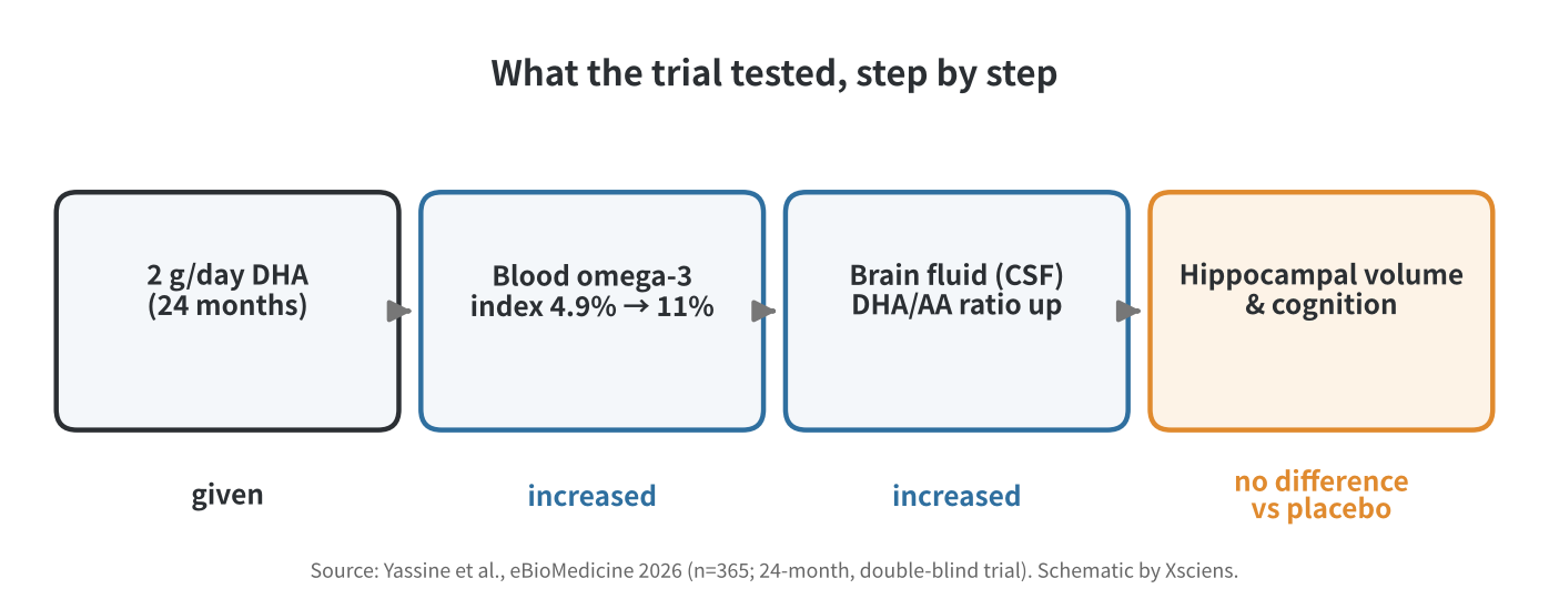
    Flow diagram: DHA given, blood omega-3 index up, brain-fluid DHA/AA ratio up, no difference in hippocampal volume and cognition
    Figure 2. The trial followed the supplement step by step; the chain broke at the last link. Schematic by Xsciens, based on Yassine et al. (2026).

    Where this fits

    Earlier randomized evidence points in the same direction. A 2012 Cochrane review of three trials, with cognitive data from 3,536 cognitively healthy adults aged 60 and over, found no cognitive benefit from omega-3 supplements. The VITAL-Cog analysis, which included 4,218 adults in two cognitive substudies, likewise found no significant effect on global cognition from 1 gram a day of marine omega-3 over about two to three years. Neither establishes whether supplements can prevent dementia itself.

    Observational research, by contrast, has suggested that people who eat more seafood may have a lower risk of cognitive decline, according to the U.S. National Center for Complementary and Integrative Health, which is one reason the question keeps being asked. For now, the evidence does not support taking high-dose DHA specifically to preserve memory in otherwise cognitively healthy older adults.

    Xsciens Editorial Note

    The core of this trial: high-dose DHA raised a brain-fluid marker, but in this group it made no measurable difference to cognition or hippocampal shrinkage.

    • Measured versus interpreted. The rise in the brain-fluid DHA-to-AA ratio was directly measured and was the trial’s primary outcome; cognition and brain volume were secondary outcomes. Both groups’ test scores rose by about 2.7 points, which could partly reflect familiarity with repeated testing, though the study cannot say how much. The finding is the absence of a group difference, not a prevented decline.
    • Limits. Roughly 38% dropout (with completers differing from dropouts), a cognitively healthy and well-educated group, a 24-month window, one dose and a phase IIa design all limit how far the result generalizes. It cannot rule out small effects, and it says nothing about dementia itself, which the trial did not measure.
    • What to watch. Whether particular groups, such as people whose brains handle DHA differently, respond better (a hypothesis, not a finding); longer follow-up with measures sensitive to decline; and replication in other populations.
    • From the editors — if you take fish oil for your memory, this trial gives you less reason to expect a payoff. The upside is a sharper research question: now that DHA is known to shift a brain-fluid marker, the next step is working out why that is not translating into better memory, and for whom. That said, this is one trial in cognitively healthy people; it does not show that omega-3 is harmful or that fish on your plate is pointless, and the lifestyle basics the lead author points to deserve at least as much of your attention as the capsule. If you take fish oil for another reason, such as heart health, talk to your doctor before changing anything.

    References for this note: Sydenham et al., Cochrane review (2012), Kang et al., VITAL-Cog (2022), NCCIH: Omega-3 Supplements

    Sources: eBioMedicine (Yassine et al., 2026), Healio, News-Medical, ScienceDaily (USC release)

  • Enzyme-Laced Plastic Stays Tough in Use, Degrades Fast in the Deep Sea

    Enzyme-Laced Plastic Stays Tough in Use, Degrades Fast in the Deep Sea

    Researchers at Japan’s New Energy and Industrial Technology Development Organization (NEDO), the University of Tokyo, the Japan Agency for Marine-Earth Science and Technology (JAMSTEC), and Gunma University have built a biodegradable plastic that keeps its strength while dry but speeds up its own breakdown once wear and water reach enzymes mixed into the material. In seafloor trials at a depth of 5,503 meters, the enzyme-laced plastic lost weight far faster than the same material without the enzymes. The team sees the work as a potential tool against marine plastic pollution, which research groups worldwide have struggled to tackle largely because so much plastic debris, once lost at sea, is effectively impossible to retrieve.

    原論文情報 / Original Paper
    原題(Title): Enzyme-embedded polyesters for accelerated biodegradation in the deep sea
    著者(Authors): QiuYuan Huang et al.
    掲載誌(Journal): Nature
    DOI: 10.1038/s41586-026-11192-1

    A Plastic Built to Switch On When Wet

    An estimated eight million tons of plastic waste enters the ocean every year, and some of it can take more than 300 years to break down in the natural environment. The same research team had previously shown, for the first time, that biodegradable plastics are broken down by microbes on the seafloor at depths of 757 to 5,552 meters — but even the fastest cases took years to fully degrade. The deep sea is cold and under high pressure, and only a limited population of microbes there is capable of breaking down this particular type of plastic, so degradation tends to be slow.

    This time, the team changed the plastic’s mechanism rather than its base material. They melted the plastic and mixed in natural degrading enzymes — HiC cutinase, which cuts polyester bonds and comes from a mold species, and CaLB lipase, an enzyme involved in fat breakdown that here was repurposed for plastic, sourced from an Antarctic yeast. These enzymes stay inactive without water, so the plastic keeps close to its original strength while dry and in use. But once wear or fragmentation in the environment lets water reach the enzymes inside, degradation accelerates from there — in effect, a plastic that switches on once it gets wet.

    It’s worth separating two related but different ideas here: how much weight a sample loses, and how completely it eventually breaks down into simpler compounds through microbial action, a process researchers call mineralization. The paper backs up its weight-loss measurements with both chemical analysis of what the enzymes actually produce and biochemical oxygen demand testing, which tracks how far seawater microbes carry that breakdown — so the result isn’t based on weight loss alone.

    Weight Loss Confirmed Even at 5,503 Meters

    The team sank plastic films at coastal sites (2 to 6 meters deep) and at several deep-sea locations — 757, 855, 1,292, and 5,503 meters — and compared how their weight changed over time. Even at 757 meters, 4°C, and 7.6 MPa of pressure (about 75 times atmospheric pressure), some of the enzyme-laced materials lost nearly all their weight within five months, versus barely any loss for the enzyme-free material over the same period. At the deepest site, 5,503 meters, enzyme-laced PBSA (polybutylene succinate adipate, hereafter PBSA) lost about 30.5% of its weight after 18 months, far more than the roughly 1.6% lost by the same material without the enzyme. Degradation varied by material, though — not every sample lost weight at the same rate, and PCL, another material in the trial, lost only about 7.7% of its weight over the same 18 months even with the enzyme added.

    Coastal seawater trials, run separately from the deep-sea deployments, told a similar story on a faster timeline: even at a lower enzyme loading of around 0.1 weight percent, several of the materials lost a substantial share of their weight within a single month in the water near shore. That matters for how the result should be read — degradation isn’t an on/off switch that waits until plastic reaches the deep ocean, but a process that speeds up as soon as water reaches the enzyme, in whatever environment that happens.

    Comparison chart of weight-loss rate for plastic with and without embedded enzyme at 5,503 m depth
    Source: created from data in Huang et al., Nature (2026)

    Fast Degradation Without Losing Strength

    A natural question is whether making the plastic easier to break down also weakens it as a product. According to the team, adding the enzyme at around 0.1 weight percent barely affects tensile strength, and even at the roughly 3 weight percent used for the deep-sea trials, the drop in strength and elongation stays within what the researchers describe as a practically usable range. Comparing weight-loss speed at 757 meters, the enzyme-laced material lost about 97 micrograms per square centimeter per day, versus just 0.9 micrograms for the enzyme-free material — a specific comparison in which the difference reached roughly 100-fold. Separately, NEDO describes the project’s overall achievement as roughly a 30-fold increase in degradation speed compared with the enzyme-free version. Both figures are accurate; they simply describe different materials and conditions rather than contradicting each other.

    Embedding the enzyme directly in the material showed that a biodegradable plastic’s weight loss can be sped up substantially, even in the deep sea, where it once degraded only very slowly.

    Micro-Sized Beads Respond Too

    The same approach was also applied to test microbeads 20 to 300 micrometers across, which degraded across a range of coastal and deep-sea conditions. This doesn’t confirm the effect in actual cosmetic-grade microbeads on the market — it’s a result from lab test particles sized to resemble microplastics. Smaller plastic particles are more likely to be taken up by marine life, and once they spread into the environment, recovering them is difficult; microbeads in particular are one of the hardest categories of marine plastic to clean up once released, since conventional filtration and collection methods struggle at that size. Building degradability into a product’s design from the start could become a new way to reduce how much plastic lingers after release. How well this translates to real products, and how much it actually reduces pollution, still needs further testing.

    Schematic showing enzyme-embedded plastic staying stable in use and degrading once it contacts water
    Source: created from NEDO news release description

    What’s Left Before Real-World Use

    The team’s next steps include testing long-term durability and safety under realistic conditions, extending the approach to a wider range of biodegradable plastics, making the enzyme-mixing process more efficient and affordable, and scaling up for mass production. Deep-sea degradation still takes several months to more than a year, so this isn’t a case of plastic vanishing the instant it’s lost. Cost is likely to be a major factor in whether the approach ever reaches store shelves, since biodegradable plastics already tend to cost more to manufacture than conventional ones, and adding a purified enzyme to the mix adds another expense on top of that. Still, compared with the several years existing biodegradable plastics have needed to break down in the deep sea, this result looks like a promising option for tackling marine plastic pollution.

    Xsciens Editorial Note

    What stands out most here is the mechanism itself: a plastic engineered to activate only once it gets wet, rather than a change to the base material.

    • “30x” and “100x” describe different comparisons. NEDO’s “about 30-fold” figure represents the project’s overall result, while the “about 100-fold” figure in this article comes from one specific comparison — weight-loss speed at 757 meters (at 5,503 meters, PBSA lost about 30.5% of its weight with the enzyme versus about 1.6% without it over 18 months; at 757 meters, the daily weight-loss rate was about 97 micrograms with the enzyme versus about 0.9 micrograms without it). Neither number is wrong, but it’s safer not to let a single multiplier stand in for every condition.
    • The materials and timescales involved have limits. The enzymes tested here work on polyester-based biodegradable plastics — PBS, PBSA, PCL, and PBAT — and don’t directly apply to everyday polyethylene or polypropylene, the materials used in most plastic bottles and bags. Deep-sea degradation still takes at least a few months, and sometimes more than a year depending on the material, so this isn’t a case of plastic disappearing the moment it’s lost.
    • Long-term, real-world testing is the next thing to watch. What’s been shown so far comes from experimental deployment trials. The research team itself lists durability and safety testing under real-use conditions, and establishing mass-production methods, as future challenges. How much this technology can actually reduce marine plastic’s buildup, while keeping costs low enough for wide adoption, remains to be seen.
    • From the editors — once this reaches the market, choosing plastic products could come with a little less guilt. Expect more everyday items — food packaging, fishing gear — built with technology like this, cutting into ocean plastic pollution without sacrificing convenience. That said, “it breaks down anyway” shouldn’t become an excuse to get careless about waste. Even as the technology improves, reducing what we throw away is still on us as consumers.

    References for this note: Chamley et al., “Polymer material biodegradation in the deep sea. A review,” Science of The Total Environment (2024), Japan Ministry of the Environment, Eco-Label Database, “Marine Biodegradable Plastics” certification program

    Sources: NEDO news release, Huang et al., “Enzyme-embedded polyesters for accelerated biodegradation in the deep sea,” Nature (2026)

  • [Science] What Is a Supramolecular Polymer? A Simple Guide to How It Works

    [Science] What Is a Supramolecular Polymer? A Simple Guide to How It Works

    A supramolecular polymer is a chain-like material whose building blocks link up through weak, reversible attractions instead of strong, fixed chemical bonds. That “weak but many” design can let these materials repair damage, change shape, and influence how living cells grow — which is why materials scientists have been racing to build bigger, more precisely controlled versions of them.

    What Is a Supramolecular Polymer?

    A conventional polymer — the plastic in a water bottle, for example — is a long chain of small repeating units called monomers, welded together end-to-end by covalent bonds. Covalent bonds are the strong, electron-sharing connections that hold most everyday molecules together, and once formed they generally don’t come apart on their own.

    A supramolecular polymer (a term built from “supra-,” meaning “beyond,” plus “molecular”) swaps those permanent welds for temporary handshakes. Its monomers link up through noncovalent interactions — hydrogen bonds, stacked ring structures, metal-ion bridges, or simple electrical attraction — that are individually weak but, strung together by the thousands along a chain, add up to a stable, functional material. A useful everyday comparison is Velcro: a single hook-and-loop pair peels apart with almost no effort, but a whole strip of them holds a heavy jacket closed. Supramolecular polymers work the same way at the molecular scale — weak links in large numbers behave like a strong, yet reversible, material.

    IUPAC’s 2013 polymer-science recommendations favor the term “supramolecular association” (also called “Lehn association,” after chemist Jean-Marie Lehn) for this self-assembly process, and discourage the related term “supramolecular polymerization.” That is a naming preference for the process, not a rejection of the material-class name: “supramolecular polymer” remains the term used throughout the chemistry and materials literature — including in the title of the 2026 Northwestern University paper described below — so this article uses it in that common sense.

    How the Self-Assembly Works

    Because the bonds holding a supramolecular polymer together are reversible, individual connections continually break and re-form, letting the material adjust to its surroundings without necessarily falling apart. When the damaged surfaces of such a material can come back into contact and the molecules are mobile enough, those reversible interactions can reconnect across the damage — the basis for self-healing in some (not all) supramolecular materials; how well it works depends heavily on the specific design. According to a 2024 overview from the Society of Plastics Engineers, this same dynamic bonding can also let certain supramolecular polymers flow or be reshaped more easily than conventional plastics, though the exact processing temperature and pressure still depend on the molecular design in question.

    Chemists have also learned to design chains that grow to a controlled length and then stop. One such strategy, demonstrated in an October 2026 study from Northwestern University, is called self-capping supramolecular polymerization. The molecular design lets a growing thread’s flexible ends keep adding building blocks while conditions allow it, then fold over and form a cap that limits further growth. Introducing a fresh batch of building blocks can restart the process, which lets researchers extend the assembly and arrange distinct segments along its length.

    Getting this right is a balancing act. If the building blocks do not bind to each other strongly enough under the given conditions, only short, unstable clusters form. If the interactions are too strong, the material can lose the ability to rearrange that makes supramolecular polymers useful in the first place. Scientists must also keep growing chains from fusing together unpredictably or slowly falling back apart — failure modes that, together with this binding-strength trade-off, are much of what makes precise supramolecular engineering difficult.

    Why It’s Getting Attention Now

    Supramolecular polymers have been studied since the late 1980s. In 1988, chemist Takuzo Aida and colleagues reported one of the field’s early milestones: disc-shaped porphyrin molecules that stacked face-to-face into one-dimensional assemblies through noncovalent interactions. Chemist Jean Fréchet’s group then used hydrogen bonds to build liquid-crystalline supramolecular structures in 1989, and Nobel laureate Jean-Marie Lehn’s group demonstrated hydrogen-bonded, liquid-crystalline supramolecular polymers in 1990. Chemist Bert Meijer’s widely cited 1997 work on four-point hydrogen-bonded monomers then showed that noncovalent assemblies could behave mechanically like true high-molecular-weight polymers. What has changed since then is precision: for decades, supramolecular polymers tended to form with uneven, hard-to-control lengths, which limited how reliably their properties could be engineered for a specific application.

    That is the gap the Northwestern team, led by materials scientist Samuel I. Stupp with postdoctoral fellow Michael Dore and graduate students Simon Egner and Madison Strong, targeted in a study published October 1, 2026, in the journal Science. Using self-capping, they built threads with molar masses reaching into the billions of daltons — roughly 100 times heavier, by the university’s own comparison, than large conventional polymers or the largest known natural proteins, with the longest threads wider than a single cell. According to the researchers, the threads kept their controlled length for months in a test tube without clumping, merging, or dissolving back apart under the tested conditions, something earlier, less-controlled supramolecular polymers struggled to do.

    “That introduces a very different way of thinking about how materials can communicate with cells,” said Northwestern’s Samuel I. Stupp of the findings.

    Diagram showing self-capping supramolecular polymerization and a charge-segmented thread anchoring to a neuron
    Source: created based on Dore et al., Science (2026) and Northwestern University’s press release.

    Uses: Self-Healing Plastics to Neurons

    The reversible bonding at the heart of supramolecular polymers already points toward several practical uses. Self-healing coatings and parts for construction, automotive, and aerospace use could extend equipment lifespans by letting small cracks mend themselves rather than requiring replacement. Stimuli-responsive versions are being explored as drug-delivery carriers that release their cargo only when they encounter a specific biological trigger, such as a change in pH inside the body, and supramolecular hydrogels — soft, water-swollen networks — are used as scaffolds in tissue engineering to support growing cells. Researchers are also testing supramolecular designs in adaptive coatings that resist corrosion and wear, and in soft robotics, where flexible, responsive materials can mimic the give-and-take of biological tissue.

    The Northwestern study adds a striking new example. The team tested several charge patterns on neurons grown in lab dishes: threads made entirely of positively charged segments harmed the cells, threads made entirely of negative segments had little effect, and randomly mixed charges produced no notable response. Only one design worked well — a short positively charged segment sandwiched between two longer negatively charged segments, which anchored the thread to the negatively charged neuron surface. In that condition, neurons showed roughly four times more measured calcium activity (an indicator of cellular signaling, though not a direct measure of overall neuronal function) after one week, and had formed more synaptic connections by two weeks, without the researchers adding any conventional biological growth factors. The researchers caution that this is cell-culture work only, with no animal or human testing yet, so any medical application for nerve repair remains a long-term prospect rather than a near-term product.

    What to Watch Next

    Market research firm Transparency Market Research estimated the global supramolecular polymer market at roughly $291.5 million in 2024, projecting about 6.5% annual growth through 2031. The more scientifically telling milestone to watch, though, is whether precisely built, billion-dalton threads like Northwestern’s can be scaled up and tested in living animals, not just lab dishes.

    For more on the specific billion-dalton threads discussed above and how they boosted nerve-cell activity in the lab, see our related article: Scientists Build a Billion-Dalton Molecular Thread Longer Than a Cell.

    Sources: Northwestern University (Weinberg College), EurekAlert! press release, IUPAC Gold Book